A Mastercard logo is seen on a credit card in this picture illustration August 30, 2017. REUTERS/Thomas White
Register now for FREE unlimited access to Reuters.com
Feb 28 (Reuters) - Mastercard has blocked multiple financial institutions from the Mastercard payment network as a result of sanction orders on Russia, it said late on Monday.
Mastercard will continue to work with regulators to abide fully by compliance obligations, the company said in a statement.
Register now for FREE unlimited access to Reuters.com
Reporting by Maria Ponnezhath in Bengaluru; Editing by Christian Schmollinger
We have received questions asking us to explain what, in our opinion, is the most private way to purchase phones on our website.
Here below is our take on the matter:
Part 1 – Acquire sound money.
Credit cards are convenient, but they’re definitely a privacy nightmare. You’re disclosing your purchases not only to the credit card company (eg: Visa, MC, etc), but to the partner bank too (unless your card is a card which is not co-branded).
Using cash would be a better proposition, but it’s confined to the physical realm, and clearly we are a web shop.
To solve the issue, you can use Monero (XMR) or Bitcoin (BTC) to pay for your phones here, and either of them is a better option from a privacy point of view.
Acquire XMR or BTC - refer to getmonero.orgorbuybitcoinworldwide.comto get an idea on various methods of acquiring them – and move it to a wallet you control
Part 2 – Get a burner sim card.
It should be pretty easy to find one at places like supermarkets, convenience stores, newsagents, and other places. Activate the sim card – you will need to give us a phone number so that the logistics company knows how to deliver the goods to you.
Part 3 – Use an address which is not your home address to get the goods.
There is no need to disclose and use an address you reside habitually. The only requirement is that you have enough access to the address you tell us so that you can retrieve your goods.
For instance, think about using your office address, your accountant / lawyer address. If you know that you’re going to move place where you live, use the address you’ll be leaving before you leave…
And that is it… if you followed the parts above, your privacy is well protected and you can go ahead and secure your private phone, in a private way.
As a representative of Ukraine in GAC ICANN, I’m sending you this letter on behalf of the people of Ukraine, asking you to address an urgent need to introduce strict sanctions against the Russian Federation in the field of DNS regulation, in response to its acts of aggression towards Ukraine and its citizens.
On the 24th of February 2022 the army of the Russian Federation engaged in a full-scale war against Ukraine and breached its territorial integrity, leading to casualties among both military staff and civilians.
By proceeding to a so-called “military operation” aiming at “denazifying” and “demilitarizing” Ukraine under the pretext of its own national security, the Russian Federation breached numerous clauses of International Law. Russia’s invasion of Ukraine is a clear act of aggression and a manifest violation of Article 2.4 of the UN Charter, which prohibits the “use of force against the territorial integrity or political independence of any State”. Also Russia is using it's weapon to target civilian infrastructure such as residential apartments, kindergartens, hospitals etc., which is prohibited by the Article 51(3) of Additional Protocol I and Article 13(3) of Additional Protocol II to the Geneva Conventions.
These atrocious crimes have been made possible mainly due to the Russian propaganda machinery using websites continuously spreading disinformation, hate speech, promoting violence and hiding the truth regarding the war in Ukraine. Ukrainian IT infrastructure has undergone numerous attacks from the Russian side impeding citizens’ and government’s ability to communicate.
Moreover, it’s becoming clear that this aggression could spread much further around the globe as the Russian Federation puts the nuclear deterrent on “special alert” and threatens both Sweden and Finland with “military and political consequences” if these states join NATO. Such developments are unacceptable in the civilized, peaceful world, in the XXI century.
Therefore, I’m strongly asking you to introduce the following list of sanctions targeting Russian Federation’s access to the Internet:
Revoke, permanently or temporarily, the domains “.ru”, “.рф” and “.su”. This list is not exhaustive and may also include other domains issued in the Russian Federation.
Contribute to the revoking for SSL certificates for the abovementioned domains.
Shut down DNS root servers situated in the Russian Federation, namely:
Saint Petersburg, RU (IPv4 199.7.83.42)
Moscow, RU (IPv4 199.7.83.42, 3 instances)
Apart from these measures, I will be sending a separate request to RIPE NCC asking to withdraw the right to use all IPv4 and IPv6 addresses by all Russian members of RIPE NCC (LIRs - Local Internet Registries), and to block the DNS root servers that it is operating.
All of these measures will help users seek for reliable information in alternative domain zones, preventing propaganda and disinformation. Leaders, governments and organizations all over the world are in favor of introducing sanctions towards the Russian Federation since they aim at putting the aggression towards Ukraine and other countries to an end. I ask you kindly to seriously consider such measures and implement them as quickly as possible. Help to save the lives of people in our country.
Also, the above was signed by the Deputy Prime Minister of Ukraine - Minister of Digital Transformation, the appendix is attached to this email.
The Kalman Filter. Helping Chickens Cross the Road.
David Austin
Grand Valley State University
I was running some errands recently when I spied the Chicken Robot ambling down the sidewalk, then veering into the bike lane. A local grocery chain needs to transport rotisserie chickens from one of its larger stores to its downtown market. Their solution? A semi-autonomous delivery vehicle that makes the three-mile journey navigating with GPS.
I was curious how this worked. The locations provided by most GPS systems are only accurate to within a meter or so. How could those juicy chickens know how to stay so carefully in the center of the bike lane?
A typical solution to problems like this is an elegant algorithm, known as Kalman filtering, that’s embedded in a wide range of technology that most of us frequently either use or benefit from in some way. The algorithm allows us to efficiently combine our expectations about the state of a system, the chickens’ physical location, for instance, with imperfect measurements about the system to develop a highly accurate picture of the system.
This column will describe some simple versions of Kalman filtering, the main observation that makes it work, and why it’s such a great idea.
A first example
Let’s begin with a simple example. Suppose we would like to determine the weight of some object. Of course, any scale is imperfect so we might weigh it repeatedly on the same scale and find the following weights, perhaps in grams.
50.4
46.0
46.1
45.1
48.9
42.6
50.7
45.7
47.8
46.7
As the result of each weighing is recorded, we update our estimate of the weight as the average of all the measurements we’ve seen so far. That is, after obtaining $z_n$, the $n^{th}$ weight, we could estimate the object’s weight by finding the average $$ x_n = \frac1n(z_1 + z_2 + \ldots + z_n). $$ The result is shown below.
As the next weight $z_{n}$ is recorded, we update our estimate:
$$
\begin{aligned}
x_{n} & = \frac1{n}\left(z_1 + z_2 + \ldots + z_{n}\right) \\
x_{n} & = \frac1{n}\left((n-1)x_{n-1} + z_{n}\right) \\
x_{n} & = x_{n-1} + \frac1{n}\left(z_{n} – x_{n-1}\right)
\end{aligned}
$$
This expression tells us how each new measurement influences the next estimate. More specifically, the new estimate $x_{n}$ is obtained from the previous estimate $x_{n-1}$ by adding in $\frac1{n}(z_{n} – x_{n-1})$. Notice that this term is proportional to the difference between the new measurement and the previous estimate with the proportionality constant being $K_n = \frac1{n}$. We call $K_n$ the Kalman gain; the fact that it decreases as we include more measurements reflects our increasing confidence in the estimates $x_n$ so that, as $n$ increases, new measurements have less effect on the updated estimates.
Suppose now that we have some additional information about the accuracy of our measurements $z_n$. For example, if $z_n$ is the chickens’ location reported by a GPS system, the true location is most likely within a meter or so. More generally, we might imagine that the true value is normally distributed about $z_n$ with standard deviation $\sigma_{z_n}$.
Returning to our weighings, we could perhaps estimate $\sigma_{z_n}$ by repeatedly weighing an object of known weight. The probability that the true value is near $z_n$ is given by the distribution
$$
p_{z_n}(x) =
\frac{1}{\sqrt{2\pi\sigma_{x_n}^2}}
e^{-(z-z_n)^2/(2\sigma_{z_n}^2)}.
$$
Let’s also suppose that we have some estimate of the uncertainty of our estimates $x_n$. In particular, we’ll assume the probability that the true value is near $x_n$ is given by the normal distribution having mean $x_n$ and standard deviation $\sigma_{x_n}$:
$$
p_{x_n}(x) =
\frac{1}{\sqrt{2\pi\sigma_{x_n}^2}}
e^{-(x-x_n)^2/(2\sigma_{x_n}^2)}.
$$
We’ll describe how we can estimate $\sigma_{x_n}$ a bit later.
These distributions could be as shown below.
Now here’s the beautiful idea that underlies Kalman’s filtering algorithm. Both distributions $p_{x_n}$ and $p_{z_n}$ describe the location of the true value we seek. We can combine them to obtain a better estimate of the true value by multiplying them. That is, we combine or “fuse” these two distributions using the product
$$
p_{x_n}(x) p_{z_n}(x).
$$
Since the product of two Gaussians is a new Gaussian, we obtain, after normalizing, a new normal distribution that better reflects the true value. In our example, the product $p_{x_n}p_{z_n}$ is shown in green.
More specifically, the product of the two distributions is
$$
\begin{aligned}
& \exp\left[-(x-x_n)^2/(2\sigma_{x_n}^2)\right]
\exp\left[-(x-z_n)^2/(2\sigma_{z_n}^2)\right] \\
& \hspace{48pt}=
\exp\left[-(x-x_n)^2/(2\sigma_{x_n})^2-(x-z_n)^2/
(2\sigma_{z_n}^2)\right].
\end{aligned}
$$
Expanding the quadratics in the exponents and recombining leads to the new normal distribution
$$
\frac{1}{\sqrt{2\pi\sigma_{x_{n+1}}^2}}
\exp\left[-(x-x_{n+1})^2/(2\sigma_{x_{n+1}}^2)\right]
$$
where
$$
\begin{aligned}
x_{n+1} & =
\frac{\sigma_{z_n}^2}{\sigma_{x_n}^2+\sigma_{z_n}^2} x_n +
\frac{\sigma_{x_n}^2}{\sigma_{x_n}^2+\sigma_{z_n}^2} z_n \\
& = x_n + \frac{\sigma_{x_n}^2}{\sigma_{x_n}^2+\sigma_{z_n}^2}(z_n –
x_n) \\
\end{aligned}
$$
Notice that this expression is similar to the one we found when we updated our estimates by simply taking the average of all the measurements we have seen up to this point. The Kalman gain is now
$$
K_n = \frac{\sigma_{x_n}^2}{\sigma_{x_n}^2+\sigma_{z_n}^2}
$$
In addition, the product of the Gaussians leads to the new standard deviation
$$
\sigma_{x_{n+1}}^2 =
\frac{\sigma_{x_n}^2\sigma_{z_n}^2}{\sigma_{x_n}^2+\sigma_{z_n}^2}
= (1-K_n) \sigma_{x_n}^2
$$
Notice that the Kalman gain satisfies $0\lt K_n \lt 1$. In the case that $\sigma_{x_n} \ll \sigma_{z_n}$, we feel much more confident in our estimate $x_n$ than our new measurement $z_n$. Therefore, $K_n\approx 0$ and so $x_{n+1} \approx x_n$, reflecting the fact that the new measurement has little influence on our next estimate.
However, if $\sigma_{x_n} \gg \sigma_{z_n}$, we feel much more confident in our new measurement $z_n$ than in our estimate $x_n$. Then $K_n\approx 1$ and $x_{n+1}\approx z_n$.
In both cases, the uncertainty in our new estimate, as measured by $\sigma_{x_{n+1}}^2 = (1-K_n)\sigma_{x_n}^2$, has decreased.
This leads to the following algorithm:
Initialize the first estimate $x_1$ and the uncertainty $\sigma_{x_1}$. We could use the first measurement as the first estimate or we could simply make a guess for the estimate and choose a large uncertainty.
Each time a new measurement $z_{n}$ arrives, update the estimate $x_{n+1}$ nd uncertainty $\sigma_{x_{n+1}}$ as follows:
Find the Kalman gain $K_n = \frac{\sigma_{x_n}^2}
{\sigma_{x_n}^2+\sigma_{z_n}^2}$.
Update our uncertainty $\sigma_{x_{n+1}}^2 =
(1-K_n)\sigma_{x_n}^2$. Since $0\lt 1-K_n\lt 1$, the uncertainty will continually decrease, which makes the algorithm relatively insensitive to the initialization.
To illustrate, suppose that we make many measurements of a known weight with our scale and determine that the standard deviation of its measurements is constant $\sigma_z=2$. Initializing so that $x_1 = z_1$ and $\sigma_{x_1} = \sigma_z = 2$, we have the following sequence of estimates along with the decreasing
sequence of uncertainties.
Tracking a dynamic system
In our first example, the quantity we’re tracking, the weight of some object, doesn’t change. Let’s now consider a dynamic process where the quantities are changing. For instance, suppose we’re tracking the height and vertical velocity of a moving object. The true height of the object could look like this, although
that true height is not known to us.
In addition to recording the height $h$, we will also track the vertical velocity $v$ so that the state of the object at some time is given by the vector
$$
{\mathbf x}_{n,n} = \begin{bmatrix} h_n \\ v_n \end{bmatrix}.
$$
The reason for writing the subscript in this particular way will become clear momentarily.
Moreover, we will assume that there is some uncertainty in both the position and the velocity. Initially, these uncertainties may be uncorrelated with one another
so that we arrive at a Gaussian
$$
\exp\left[-(h-h_n)^2/(2\sigma_{h_n}^2) –
(v-v_n)^2/(2\sigma_{v_n}^2)\right]
$$
that describes the multivariate normal distribution of the true state. A more convenient expression for this Gaussian uses the covariance matrix
$$
P_{n,n} = \begin{bmatrix} \sigma_{h_n}^2 & 0 \\
0 & \sigma_{v_n}^2 \\
\end{bmatrix}
$$
so that the Gaussian is defined in terms of the quadratic form associated to $P_{n,n}^{-1}$:
$$
\exp\left[-\frac12 ({\mathbf x} – {\mathbf x}_{n,n})^TP_{n,n}^{-1}({\mathbf x} –
{\mathbf x}_{n,n})\right].
$$
The following figure represents the value of this distribution by shading more likely regions more darkly.
Now if we know $x_{n,n}$, the state at some time, we can predict the state at a later time using some assumption about the system. For instance, we might assume, after $\Delta t$ time units have passed, that the new state is ${\mathbf x}_{n+1,n} = \begin{bmatrix}h_{n+1} \\ v_{n+1} \end{bmatrix}$ where
$$
\begin{aligned}
h_{n+1} & = h_n + v_n\Delta t \\
v_{n+1} & = v_n.
\end{aligned}
$$
That is, we assume that the height has increased at the constant velocity given by the state vector ${\mathbf x}_n$ and that the velocity has remained constant. More succinctly, if
$$
F_n = \begin{bmatrix} 1 & \Delta t \\ 0 & 1 \end{bmatrix},
$$
we can write
$$
{\mathbf x}_{n+1, n} = F_n{\mathbf x}_{n}.
$$
The subscript ${\mathbf x}_{n+1, n}$ reflects the fact that we are extrapolating the next state using information only from the previous state.
This is a particular model we are choosing; in other situations, another model may be more appropriate. For instance, if we have information about the object’s acceleration, we may want to incorporate it. In any case, we assume there is a matrix $F_n$ from which we extrapolate the next state:
$$
{\mathbf x}_{n+1,n} = F_n{\mathbf x}_{n,n}.
$$
Of course, uncertainty in the state ${\mathbf x}_{n,n}$ will translate into uncertainty in the extrapolated state ${\mathbf x}_{n+1,n}$. It is straightforward to verify that the covariance matrix is transformed as
$$
P_{n+1,n} = F_nP_{n,n}F_n^T.
$$
For instance, if the uncertainties in position and velocity are initially uncorrelated, they may become correlated after the transformation, which is to be expected.
These two transformations form the extrapolation phase of the algorithm:
$$
\begin{aligned}
{\mathbf x}_{n+1,n} & = F_n{\mathbf x}_{n,n} \\
P_{n+1,n} & = F_nP_{n,n}F_n^T.
\end{aligned}
$$
Next, suppose we have a new measurement ${\mathbf z}_{n}$ whose uncertainty is described by the covariance matrix $R_{n}$. We imagine that the normal distribution centered on ${\mathbf z}_{n}$ and with covariance matrix $R_n$ describes the distribution of the true state.
As before, we will fuse our predicted state ${\mathbf x}_{n+1,n}$ with the measured state ${\mathbf z}_{n}$ by multiplying the two normal distributions and rewriting as a single Gaussian. With some work, one finds the expression for the Kalman gain $$ K_{n} = P_{n+1,n}(P_{n+1,n} + R_{n})^{-1}, $$ which should be compared to our earlier expression.
We also obtain the updated state and covariance matrix
$$
\begin{aligned}
{\mathbf x}_{n+1, n+1} & = {\mathbf x}_{n+1,n} + K_{n}({\mathbf z}_{n} –
{\mathbf x}_{n+1,n}) \\
P_{n+1,n+1} & = P_{n+1, n} – K_{n}P_{n+1,n}. \\
\end{aligned}
$$
So now we arrive at a new version of the algorithm:
Initialize the initial state ${\mathbf x}_{1,1}$ and covariance matrix $P_{1,1}$.
As new measurements become available, repeat the following steps:
Form the extrapolated state and covariance:
$$
\begin{aligned}
{\mathbf x}_{n+1,n} & = F_n{\mathbf x}_{n,n} \\
P_{n+1,n} & = F_nP_{n,n}F_n^T.
\end{aligned}
$$
Use the result to find the Kalman gain
$$
K_{n} = P_{n+1,n}(P_{n+1,n} + R_{n+1})^{-1},
$$
Use the Kalman gain to fuse the predicted state with the measured state and update the covariance matrix.
$$
\begin{aligned}
{\mathbf x}_{n+1, n+1} & = {\mathbf x}_{n+1,n} + K_{n}({\mathbf z}_{n} –
{\mathbf x}_{n+1,n}) \\
P_{n+1,n+1} & = P_{n+1, n} – K_{n}P_{n+1,n}. \\
\end{aligned}
$$
Let’s see how this plays out in an example. Imagine we are tracking the height and vertical velocity of an object whose true height as is shown.
Remember that we don’t know the true height, but we do have some noisy measurements that reflect the object’s height and its velocity.
Applying the Kalman filtering algorithm naively, we obtain the green curve describing the object’s height. Notice how there is a time lag between the filtered height and the true height.
What’s the problem here? Clearly, the object is experiencing a significant amount of acceleration, which is not built into the model. As we saw in our earlier static example, the uncertainty in the estimated state ${\mathbf x}_{n,n}$ continually decreases, which means the confidence we have in our estimates grows and causes us to downplay the new measurements.
There are several ways to deal with this. If we have measurements about the acceleration, we could rebuild our model so that the state vector ${\mathbf x}_{n,n}$ includes the acceleration in addition to the position and velocity. Alternatively, if we have information about how an operator is controlling the object we’re tracking, we could build it into the extrapolation phase using the update
$$
{\mathbf x}_{n+1,n} = F_{n}{\mathbf x}_{n,n} + B_n{\mathbf u}_n
$$
where ${\mathbf u}_n$ is a vector describing some additional control and $B_n$ is a matrix describing how this control feeds into the extrapolated state. Clearly, we need to know more about the system to incorporate a term like this.
Finally, we can simply build additional uncertainty into the model by adding it into the extrapolation phase. For instance, we could define
$$
P_{n+1,n} = F_nP_{n,n}F_n^T + Q_n,
$$
where $Q_n$ is a covariance matrix known as process noise and represents our way of saying there are additional influences not incorporated in the extrapolation model:
${\mathbf x}_{n+1,n} = F_n{\mathbf x}_{n,n}$.
Adding some process noise into the extrapolation phase prevents us from becoming overly confident in the extrapolated states and continuing to give sufficient weight to new measurements. This leads to the filtered state as shown below, which is clearly much better than the measured signal.
Summary
Kalman developed this algorithm in 1960, though it seems to have appeared earlier in other guises, and found a significant early use in the Apollo guidance computer. Indeed, the algorithm is well suited for this application. While the guidance computer was a marvel of both hardware and software engineering, its memory and processing power were modest by our current standards. As the algorithm only relies on our current estimate of the state, its demands on memory are slight, and the computational complexity is similarly small.
In addition to being fast and efficient, the algorithm is also optimal in the sense that, under certain assumptions on the system being modeled, the algorithm has the smallest possible expected error obtained from a given set of measurements.
Kalman filtering is now ubiquitous in navigation and guidance applications. In fact, it is used to smooth the motion of computer trackpads so you may have used it while reading this article. If you are driving while navigating with an app like Google Maps, you may notice the effect of the algorithm when you come to a stop at a traffic light. It sometimes happens that your location continues with constant speed into the intersection and then quickly snaps back to your actual location. The extrapolation phase of the algorithm would lead us to believe that we continue with constant speed into the intersection before new measurements pull the extrapolated locations back to our true location.
There are lots of relevant references on the internet, but few give an intuitive sense of what makes this algorithm work. Besides Kalman’s original paper, I’ve given a few of those here.
Australia's national intelligence agencies have dismissed concerns surrounding laws currently before Parliament that would provide them with expanded data-gathering powers in circumstances where an Australian person's safety is in imminent risk.
The Bill in question, if passed, would enable national intelligence agencies to undertake activities to produce intelligence where there is, or is likely to be, an imminent risk to the safety of an Australian person, such as from terrorist attacks or kidnappings.
It would also allow these agencies to seek ministerial authorisation to produce intelligence on Australians involved with a listed terrorist organisation rather than having to obtain multiple, concurrent authorisations to produce intelligence on individual Australian persons who are suspected of being involved with a listed terrorist organisation.
Opposition of the Bill has primarily come from the Law Council of Australia (LCA), which told the Parliamentary Joint Committee on Intelligence and Security (PJCIS) it was unsure whether the expanded powers would be proportionate to their operational objectives.
In a submission to the PJCIS, which is responsible for scrutinising Australia's intelligence powers, the LCA said there are no safeguards to prevent agency heads from using its intelligence-gathering powers on an Australian in situations where they are not in imminent risk.
"There is no requirement that the agency head must also assess the nature and degree of the imminent risk to the person's safety, and be satisfied that it is sufficiently serious as to warrant the exercise of powers in the absence of a ministerial authorisation," LCA wrote in its submission to the committee.
"For example, there is no requirement to be satisfied that there is a risk of death or serious harm to the person."
The LCA added it was also concerned about expanding the influence of a single ministerial authorisation so it can enable intelligence-gathering of entire terrorist organisations due to the broad nature of such an authorisation.
The council specifically noted the lack of an exhaustive list for what is deemed to be "involvement with a listed terrorist organisation".
"The Law Council notes that the concept of a person's 'involvement with' a listed terrorist organisation has the potential to be extremely broad, covering both direct and indirect forms of engagement," it said.
"The Law Council suggests that consideration is given to placing more precise statutory parameters on the concept of 'involvement with' a listed terrorist organisation."
In response to these concerns, representatives from the Department of Home Affairs, Australian Security Intelligence Organisation, Australian Signals Directorate (ASD), and the Office of National Intelligence said these expanded powers would only be used in "niche circumstances".
"In an operational sense, when we kind of try to apply these new provisions to real-world situations what we're trying to do is save minutes and possibly hours in operational circumstances where an Australian person has been kidnapped overseas," ASD Director-General Rachel Noble said, when explaining the "imminent risk" powers.
Noble said waiting for ministerial authorisations is not always possible in "imminent risk" situations as overseas kidnappings and mass casualty events can often occur in the middle of the night.
Addressing the LCA's concern regarding ministerial authorisations potentially being too broad for gathering intelligence on listed terrorist organisations, a Home Affairs representative said the authorisations would only be used by intelligence agencies to investigate members of the class that directly participate in listed terrorist organisations.
Home Affairs electronic surveillance assistant secretary Paul Pfitzner said authorisations for agencies to perform intelligence activities on a listed terrorist organisation would only allow them to investigate individuals who recruit others, provide and receive training, provide financial or other forms of support, and advocate on behalf of the organisation.
"We don't want to pretend that we'll necessarily be able to capture every scenario, situation, or circumstance that might arise in the course of an intelligence agency undertaking their work and finding how people may or may not be involved with a particular terrorist organisation," Home Affairs electronic surveillance first assistant secretary Andrew Warnes added.
In terms of accountability, Pfitzner said all intelligence agencies who collect data about terrorist organisation individuals through ministerial authorisations would have to keep a list of these identified individuals and provide reasons why they are classified as being part of those organisations.
Related Coverage
from Latest Topic for ZDNet in... https://ift.tt/7sCma1Z
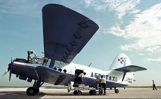
Retired from the Hungarian Air Force, the An-2 acquired in 1989 by the Planes of Fame Air Museum in Chino, California, lumbered over the landscape on exhibition flights. Today, it’s on static display. Philip Makanna
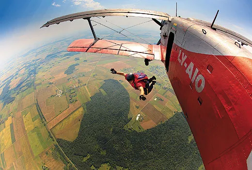
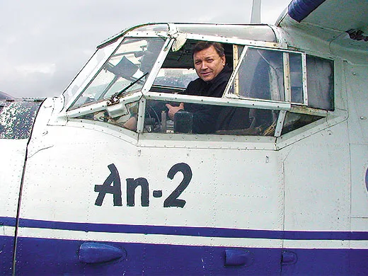
I have taken off in Antonov An-2 biplanes more than 100 times, but never landed in one. Since the late 1950s, the big Russian biplanes have carted skydivers like me aloft from jump bases all over the world—but not in the United States.
Although almost 19,000 An-2s were produced in the Soviet Union, China, and Poland, and the airplane has been certified in more than 20 countries (including Germany, Brazil, and Iraq), the An-2s that made it to the United States after the collapse of the Soviet Union will not haul jumpers or any other passengers to earn money. They won’t spray crops, as they do in other countries, carry cargo, or fight fires. The U.S. Federal Aviation Administration restricts An-2s to pleasure flights and airshow flybys, a limitation akin to turning a draft horse into a house pet.
I learned to skydive in February 1990, at a Soviet military base in Volosova, an hour south of Moscow. Back then, the U.S.S.R. was edging toward disintegration, and An-2s had alreadybegun. The base was home to a fleet of Antonovs and more than a dozen helicopters. At first, the base commander decided to sell several airplanes in order to keep buying fuel and food. Then a bigger idea caught hold: Within a couple of years, he had divested the place of a few more An-2s and a couple of helos and built a pretty snazzy hotel, which he ran as a resort for skydivers from around the world.
When chaos descended on the U.S.S.R., Iouri Kharitonov, a compact, energetic, convivial fellow with more than 9,500 hours in An-2s, was flying for a small regional air service in the Soviet far east, part of the gargantuan national Aeroflot conglomerate. “It was wild,” says Kharitonov of the Soviet breakup. “There were no laws. Nobody knows what rules to follow.”
At first, Kharitonov attempted to set up his own company, continuing to fly passengers and supplies to remote villages around Magadan, a port on the Okhotsk Sea, north of Japan, as he had done as an Aeroflot employee. The Antonov can carry 12 passengers or up to 3,500 pounds of cargo. “But the airplanes were junk,” says Kharitonov, and the business failed.
Steve Thomson, who reports on Russian aviation from Scotland for Concise Aerospace, a Web site that has covered the industry for business execs since 1992, traveled in Russia in the mid-1990s. “It’s hard to express how completely uncontrolled the situation was,” he says. “It was massively corrupt. I could have bought anything—airplanes, tanks. Airplanes just disappeared from registers and went to private individuals.”
These liberated aircraft went cheap, and about 100 made their way to the United States, crossing the north Pacific and Bering Sea from places like Khabarovsk and Petropavlovsk, in eastern Russia.
Al Stix, a part owner in the Creve Coeur airport near St. Louis, Missouri, and collector of vintage airplanes, bought an Antonov in 1989, which came by a different route. His is the penultimate airplane built at a factory in Mielec, Poland, which produced almost 12,000 An-2s under license, beginning in 1959.
“Mine was a legit deal,” says Stix, “but a lot of them got winkled out of Soviet Russia about the time that country fell apart. It’s pointless to ask about where exactly they came from because no one kept any paper trail, if one ever existed.”
We do know, however, where 10 of them came from.
In 1996, with two partners, Iouri Kharitonov bought 10 An-2s from Aeroflot at a bargain-basement price. “The price was very low because in Russia nobody could operate them,” says Kharitonov. “The avgas disappeared and nobody produces it any more.”
“Refineries weren’t producing the fuel,” agrees Steve Thomson, and in the mid-1990s, he says, “imported fuel cost four times what it had cost in the Soviet Union.”
Kharitonov and his partners wanted to get their airplanes to the United States, where fuel was plentiful and relatively cheap, but they were starting in Russia, where fuel was scarce and expensive. Flying one An-2, which at cruising speed consumes 43 gallons of fuel an hour, would have been difficult; flying 10 of them would have been prohibitive. The group decided to remove the wings and props from their fleet and ship them across the Pacific from Vladivostok. In 1996, Kharitonov and the Antonovs arrived in Tacoma, Washington.
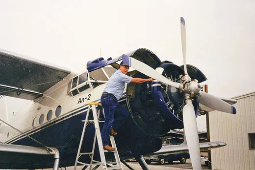
Upon clearing customs in Tacoma, Kharitonov trucked the shipping containers to the Auburn, Washington, airport where he reassembled the aircraft and planned to form a company for aerial firefighting and crop dusting.
Two FAA advisors oversaw the reassembly, and Kharitonov recalls calming their doubts about the airworthiness of the craft by promising to take his mechanics on all the maiden flights of the rebuilt biplanes. He replaced the weather-worn cotton fabric on the wings with American polyfiber. “The first reassembly took several days, but by the 10th we could do one a day,” Kharitonov recalls, adding, “The people at the Auburn airport were great to work with and very encouraging. I think they liked having them just to look at.”
The giant biplanes are an arresting sight. The upper wing spans almost 60 feet, and the wings are separated by seven feet. The lower wing spans 46 feet, 8.5 inches. The four-blade variable pitch propeller is nearly 12 feet in diameter. The cargo compartment in the 42-foot-long fuselage can easily accommodate 12 parachutists and their equipment, with two rows of seats that fold down and face each other.
In Volosova, I discovered that the aircraft are the perfect platforms to jump from. When the engines started, they sounded like a gaggle of unmuffled Harleys, but takeoffs, especially on the ski-equipped airplanes, were so smooth that if you weren’t looking out a window you wouldn’t know you were in the air. Climbing in an An-2 is like ascending in a grain bin; the thin aluminum of the fuselage, padded by your parachute, transfers the vibrations, and shakes you like one of those two-bit massage beds of cold war-era motels. You’re sitting sideways and leaning slightly aft until the tail lifts and flies serenely for a few seconds of equipoise, then you’re in the air and the big prop digs in and yanks you up to 10,000 feet in a few minutes. Finally, at a cruising speed that feels about as challenging as the wind in your hair at a sprint, you step into the prop wash. I’d want to wing walk one of these big dragons, but for their fabric skins.
“It’s very stable,” says airline pilot J.D. Webster. In 1996, Webster bought two of the Antonovs that Kharitonov had shipped to Tacoma. “Some pilots have told me that it handles very much like a DC-3,” he says. Webster, whose mother was born in Guatemala, had long thought of starting a small air service there. “I’ve spent a lot of time in Guatemala,” he says, “and I always felt that the transportation system was underdeveloped. After seeing the An-2, I thought Wow, that might work.” With a third An-2 bought from a broker in Florida, Webster started a tiny airline to carry cargo and passengers to remote villages. Kharitonov eventually became a partner in the business.
“There’s nothing like them for landing heavy loads on short strips,” says Webster’s father John, who hopped rides on his son’s aircraft and maintains an2flyers.org, a Web site for An-2 owners and fans.
J.D.’s airline established the Antonov’s bush cred in Guatemala during Hurricane Mitch, when for three days in 1998 the aircraft was the only means of getting food and water to 5,000 families on a banana plantation. “You could land that thing anywhere,” says J.D., noting that once, in the States, he took off in less than 75 yards and on landing, stopped in under 100 feet. But by the end of 2001, a combination of government hassle and changes in regulations shut his small business down.
Before his Guatemalan adventure, J.D. snagged a U.S. Navy contract to fly one of his airplanes as a radar target. In this test, the airplane demonstrated another of its celebrated characteristics: its ability to fly unbelievably slow before stalling. “We lumbered along at 60 knots [about 70 mph], maintaining altitude so the Navy could capture the radar signature,” he says. The test, run out of Naval Air Station Point Mugu in California, was meant to support the sale of F-15s to South Korea by proving that the radar—built by Lockheed Martin and used at the time on the Navy’s F-14 Tomcats—could track slow Antonovs, which the North Koreans flew in the 1990s to transport commando paratroopers. “We flew 30 or 40 miles out to sea in the Pacific Missile Test Range to rendezvous with an F-14,” says Webster. “The F-14 got back to base in about 10 minutes. It took us 45.”
The controllers at the base tower were accustomed to jets; “they couldn’t figure out what we were,” Webster says. “When they started tracking us, I got a call saying ‘What are you? Are you a helicopter?’ ”
“It will fly a lot slower than that,” says John Webster. Along for a ride in Guatemala in 1997, when Kharitonov demonstrated the airplane’s stall behavior for the pilots in the start-up air service, Webster was astonished when Kharitonov flew at such a slow speed—around 35 mph—that the airspeed indicator stopped working. He was demonstrating a landing in what Webster calls “the parachute mode,” which entails stalling the aircraft down low and having it drop onto the field. “You might bend the airplane,” says Webster, “but you’d walk away.” The Antonov’s operator’s handbook doesn’t bother to list a stall speed. Pilots could control it at such slow speeds that Soviet paratroopers would practice low-level jumps into snowdrifts without parachutes.
But for all its utility, the Antonov’s birth on the wrong side of the Iron Curtain keeps it from working in the United States—something Kharitonov learned only after arriving here.
While the Soviet Union was dissolving and surplus military equipment began pouring into the United States, the FAA, according to a spokesman’s e-mail, “developed advisory materials to inform the public of the difficulties of purchasing and certifying certain former military aircraft. FAA Advisory Circular AC 20-96 is an example of such advisory material.” There it is in black and white: “Many surplus military aircraft do not conform to any existing civilian type certificate, and some can never be made to conform, regardless of the effort and money expended to modify the aircraft.” But Kharitonov had flown Antonovs in civil service; small wonder that an advisory entitled “Surplus Military Aircraft: A Briefing for Prospective Buyers” didn’t alert him to the problem. Bottom line: If the FAA itself has not awarded a type certificate—design approval issued to an applicant who has demonstrated that a product complies with the applicable airworthiness standards and regulations—the airplane cannot receive a standard airworthiness certificate. The only operator’s certificate available to Kharitonov was an “experimental” certificate, which prevents him from flying the firefighting and crop- dusting jobs at which he’d hoped to make a living. The experimental certificate prohibits him from flying more than 25 miles from home without notifying the FAA. “That being a federal law, it has essentially grounded every An-2 in the U.S.,” he says. “Finally I said, ‘Give me that stupid experimental certificate.’ I keep one airplane for me to fly.”
The FAA has not singled out the Antonov for special treatment. At the same time An-2s were coming in from former Warsaw Pact countries, dozens of Czech Aero L-39 and L-29 jet trainers were migrating to the United States. All of those jets have experimental certifications too.
“I didn’t bring the airplanes here to sell them,” says Kharitonov. But that’s what he has done. Today, he earns a living by driving a limousine in Seattle. “I have the last few planes for sale for less than what their propellers would cost,” he adds. They are advertised on an2flyers.org.
The site lists 240 An-2s registered in 44 countries—and that number reflects only the aircraft whose owners submitted information. John Webster includes on the site his personal tips on Antonov maintenance, including “How to service cowl flap motor brushes without removing engine using two skinny guys with long arms.”
One of the owners not registered on Webster’s Web site is Michael Kimbrel. “I always wanted one because I could haul my wife and 15 kids in it,” says Kimbrel, 68, a lanky recluse of the John Wayne mold, who requests that I not disclose the location of his stable of exotic airplanes. Kimbrel, a retired Delta Air Lines captain, has been flying for 50 years and still freelances as a corporate jet pilot. He bought his An-2 for “a little north of 35 grand,” he says, and might have had misgivings about purchasing it had he known that the only operating certificate offered by the FAA would be “experimental.”
The huge biplane inside his hangar has several other airplanes tucked in under it. (J.D. Webster was impressed that the landing gear struts were just long enough to allow mechanics to roll a 50-gallon drum of fuel under the airplane when it was time to gas up on unimproved airstrips.) “Here’s an aircraft that can do anything a Cessna Caravan can do. It competes with the [de Havilland] Otter’s capabilities,” says Kimbrel, who, like other Antonov owners, grumbles about a conspiracy of U.S. airplane-maker lobbyists influencing the FAA’s decision to deny a type certificate to the An-2 in order to keep it from competing with homegrown airplanes. “Actually there probably isn’t any other plane in its class,” Kimbrel says. “If John Deere were to build an airplane, this is about what they’d come up with,” he says. Indeed, the Antonov on Kimbrel’s farm smells strongly of agricultural chemicals.
Al Stix knew when he bought his An-2 that he wouldn’t be able to certify it for passengers and other commercial uses, but, he says, “This airplane is a blast to fly. It doesn’t do a thing for you. You can’t take your hands off the controls for more than a few seconds, but nothing happens too fast in a plane this big. It’s a sloppy puppy and a gas hog.”
He especially loves landing his An-2: “You’re sitting as high as a commercial airline pilot and you want to flare because you’re going so slow—the theoretical stall speed is 22 knots. So you pull back on the yoke, but the damn airplane starts to climb! They have real good landing gear and every landing I’ve made was beautiful.” Creve Coeur Airport got a second An-2 about five years ago, when a friend donated the aircraft to Stix’s Historic Aircraft Restoration Museum.
In a hair-raising memoir, Antonovs Over the Arctic, Robert Mads Anderson tells of his flight from Anchorage to the North Pole with adventurer Shane Lundgren and four other pilots in a pair of An-2s. With auxiliary tanks aboard, the two crews would stay aloft for more than 22 hours, the huge propellers digging into the air like maniacal kayak paddles. The teams installed helicopter wind speed indicators because, in a 30 mph headwind, the An-2 would practically hover.
The Antonov exodus isn’t over. A recent post on John Webster’s Web site listed an airworthy An-2 in Lithuania for $25,000. Delivered to a U.S. port unassembled, the price rose to $38,500. The biplanes that have hauled cargo, military and civilian passengers, farm harvests, pesticides, and fire retardants since 1948 still carry these and numerous other 3,500-pound loads in countries around the world.
Tom Harpole is a writer in Montana. His first story for Air & Space was about learning to skydive from an Antonov An-2.
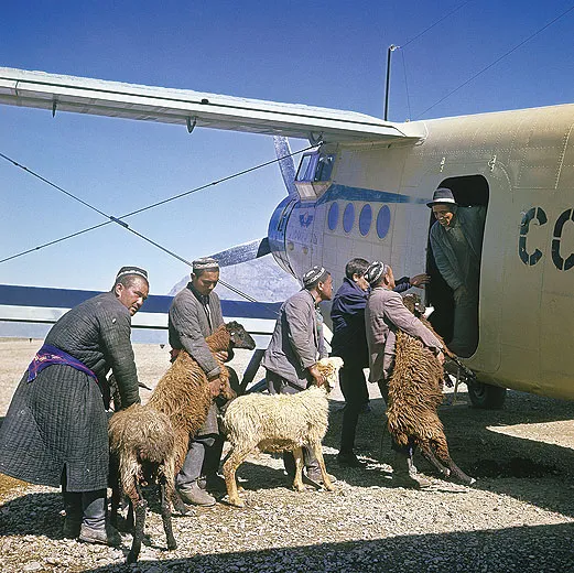
In 1967 Uzbekistan, sheep traveled by An-2. Rianovosti
Retired from the Hungarian Air Force, the An-2 acquired in 1989 by the Planes of Fame Air Museum in Chino, California, lumbered over the landscape on exhibition flights. Today, it’s on static display. Philip Makanna
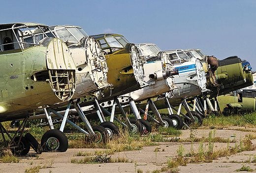
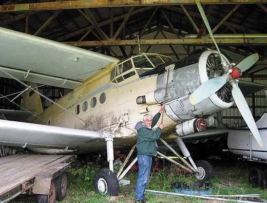
Of the more than 5,000 built in the Soviet Union, hundreds still fly; a like number, having donated engines and parts, disintegrate at Russian repair facilities. Stephan Karl
In Lithuania, an An-2 does what the type does best. Vidas Kaupelis
In Mexico, another delivers packages. Fernando Rodriguez Zapata
Iouri Kharitonov had hoped to fly An-2s in the United States on similar jobs. Vladimir Ursachil
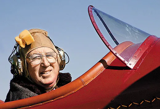
Vintage airplane collector Al Stix is content with the An-2’s all-play-andno- work U.S. status. Don Parsons
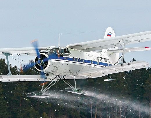
In snowy Stavropol, Russia, skis help a Polish-built Antonov perform its famous magic: short takeoff. Sergey Ryabtsev
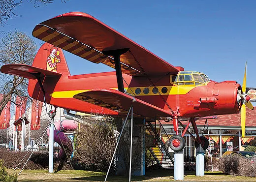
John Webster tracks sales of An-2s around the world, but even he could not have predicted this job for an An-2 on Kerepesi Street in Budapest, Hungary, where three McDonald’s restaurants advertise their locations with the giant biplanes. Courtesy John Webster
John Webster tracks sales of An-2s around the world, but even he could not have predicted this job for an An-2 on Kerepesi Street in Budapest, Hungary, where three McDonald’s restaurants advertise their locations with the giant biplanes. Szabo Gabor
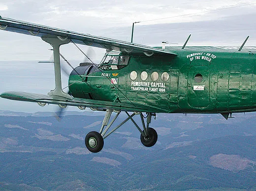
One of two Antonovs that landed at the North Pole in 1998 is on exhibit today at Seattle’s Museum of Flight. Janet Cathcart
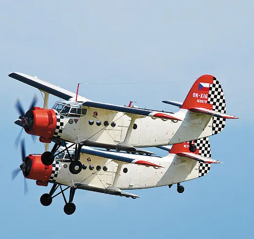
Still working in Russia in 2007, an An-2 sprays a field near Stavropol, but in the Czech Republic, an aviation club flies twin Antonovs just as U.S. pilots do: only to celebrate the survival of a remarkable airplane. Vladimir Tonkikh
Antonov owner Michael Kimbrel takes a swipe at the dust that has collected on his now-inactive biplane. Courtesy Michael Kimbrel
Still working in Russia in 2007, an An-2 sprays a field near Stavropol, but in the Czech Republic, an aviation club flies twin Antonovs just as U.S. pilots do: only to celebrate the survival of a remarkable airplane. Pavel Zhuravkov
I like to learn at least one new programming language every year - it’s mostly for fun - they are rarely useful for projects that I actually have to ship. This year, I’ve decided to look at Zig. After skimming through the official documentation and finishing the ray tracing in one weekend exercise, I realize that Zig can help with my game even though it has zero lines of Zig code.
A little background information. Most of the gameplay code is written in the game engine’s scripting environment in TypeScript. But there are a few native binaries that I need to ship as well. Given the game supports six platforms: Windows, Mac, Linux, Web, iOS, and Android, this process is quite tedious (although usually these binaries are only needed for a subset of platforms)
Currently, I do not use a cross-platform compilation toolchain - because they are hard to set up and have a lot of issues. Instead, I set up a toolchain for each target platform (I need it anyway to ship the game executable), compile the binary, put it in the repository, and call it a day. It’s not an elegant solution but it works - as long as I don’t update them very often.
Compile C with Zig
Zig has a decent cross compilation support. Not only that, it also provides a way to build C code: zig cc
Let’s try with an example project. Duktape is an embeddable JavaScript engine with a small footprint, written in C99. Since Windows is my main development environment, there are two choices: MSVC or MinGW(GCC/Clang). Each involves gigabytes of downloads and a complex installation process.
Compared to that, setting up Zig is simple: download the prebuild binary for Windows, extract in a directory, add zig executable to PATH and we are good to go.
Now we can try to compile the example that comes with DukTape. Here’s the command to do that in the official documentation:
So we can replace gcc with zig cc(Note: I am using Git Bash/MinGW64 shell)
zig cc -std=c99 -o hello -Isrc src/duktape.c examples/hello/hello.c -lm
The command finishes without an error - that’s a good sign. Let’s try to run it
$ ./hello
Illegal instruction
Oops, that doesn’t look good. After some googling, it turns out that by default, zig will pass -fsanitize=undefined -fsanitize-trap=undefined to Clang, which will cause undefined behavior (UB) to generate “illegal instruction”. In the DukTape code, there are some UB but since our purpose is not to fix it (we have a game to ship!), let’s ignore it for now by adding -fno-sanitize=undefined
zig cc -std=c99 -o hello -Isrc src/duktape.c examples/hello/hello.c -lm -fno-sanitize=undefined
Now it looks better!
$ ./hello
Hello world!
2+3=5
This is very impressive considering all I need is a ~60MB self-contained Zig compiler on the Windows platform. But it’s not only that - zig cc also supports cross-compilation out of the box.
Cross Compilation
Let’s try compiling the same code on Windows for macOS. This can be achieved by simply adding a target
Then copy the binary to my Macbook Pro (Intel), make it executable, and run it
% chmod +x ./hello
% ./hello
Hello world!
2+3=5
It just works!
Working With C in Zig
At this point, my game, which has zero line of Zig code, can already benefit from the wonderful toolchain that Zig comes with. But since we are here, let’s maybe convert some of the C code to Zig - after all Zig is a more modern language and is much more pleasant to use.
We can use zig init-exe to initialize an empty Zig project template. We will get a build script build.zig and a main source file src/main.zig. To use Duktape in this Zig project, let’s copy duktape.cduktape.h and duk_config.h to src/vendor. There are two main approaches to import C code: @cImport and zig translate-c. They both utilize the same underlying infrastructure but the latter offers more flexibility.
First, we need to translate duktape.h to Zig and write it to a file
zig translate-c -lc duktape.h > duktape.zig
Then we can simply import the Zig file in our main
conststd=@import("std");constduktape=@import("vendor/duktape.zig");pubfnmain()!void{constctx=duktape.duk_create_heap_default();constcode=duktape.duk_peval_string(ctx,"5+1");std.log.info("peval result code = {}",.{code});constresult=duktape.duk_get_int(ctx,-1);std.log.info("peval result = {}",.{result});}
Another benefit of zig translate-c is that we can get some nice IntelliSense support from IDE/Editor via Zig Language Server.
To run our project, we need to modify the build script. The default project template should have a section that looks like this:
This looks complicated at first but after some digging, we can see that duk_create_heap accepts an optional function type, but NULL, which is used for bridging C’s NULL, cannot be coerced into that - thus the complaint from the compiler. There’s in fact an open issue about this. If we look at duktape.h source file, it looks like this
$ zig build run
info: peval result code = 0
info: peval result = 6
Conclusion
Traditionally, if I need to work with C files but want some batteries included, C++ is the language to go to. C++ has a large feature set and a heavy toolchain but most of the time, I only use a small subset of features. Plus C++ doesn’t spark joy.
Zig fills this niche nicely. It is easy to set up, has a modern toolchain and build system that works well on different platform. It comes with cross-compilation support out of the box. The language is easy to pick up and an absolute joy to work with. If you don’t need the sledgehammer that is C++, give Zig a try.
by Meta AI - Donny Greenberg, Colin Taylor, Dmytro Ivchenko, Xing Liu
We are excited to announce TorchRec, a PyTorch domain library for Recommendation Systems. This new library provides common sparsity and parallelism primitives, enabling researchers to build state-of-the-art personalization models and deploy them in production.
How did we get here?
Recommendation Systems (RecSys) comprise a large footprint of production-deployed AI today, but you might not know it from looking at Github. Unlike areas like Vision and NLP, much of the ongoing innovation and development in RecSys is behind closed company doors. For academic researchers studying these techniques or companies building personalized user experiences, the field is far from democratized. Further, RecSys as an area is largely defined by learning models over sparse and/or sequential events, which has large overlaps with other areas of AI. Many of the techniques are transferable, particularly for scaling and distributed execution. A large portion of the global investment in AI is in developing these RecSys techniques, so cordoning them off blocks this investment from flowing into the broader AI field.
By mid-2020, the PyTorch team received a lot of feedback that there hasn’t been a large-scale production-quality recommender systems package in the open-source PyTorch ecosystem. While we were trying to find a good answer, a group of engineers at Meta wanted to contribute Meta’s production RecSys stack as a PyTorch domain library, with a strong commitment to growing an ecosystem around it. This seemed like a good idea that benefits researchers and companies across the RecSys domain. So, starting from Meta’s stack, we began modularizing and designing a fully-scalable codebase that is adaptable for diverse recommendation use-cases. Our goal was to extract the key building blocks from across Meta’s software stack to simultaneously enable creative exploration and scale. After nearly two years, a battery of benchmarks, migrations, and testing across Meta, we’re excited to finally embark on this journey together with the RecSys community. We want this package to open a dialogue and collaboration across the RecSys industry, starting with Meta as the first sizable contributor.
Introducing TorchRec
TorchRec includes a scalable low-level modeling foundation alongside rich batteries-included modules. We initially target “two-tower” ([1], [2]) architectures that have separate submodules to learn representations of candidate items and the query or context. Input signals can be a mix of floating point “dense” features or high-cardinality categorical “sparse” features that require large embedding tables to be trained. Efficient training of such architectures involves combining data parallelism that replicates the “dense” part of computation and model parallelism that partitions large embedding tables across many nodes.
In particular, the library includes:
Modeling primitives, such as embedding bags and jagged tensors, that enable easy authoring of large, performant multi-device/multi-node models using hybrid data-parallelism and model-parallelism.
Optimized RecSys kernels powered by FBGEMM , including support for sparse and quantized operations.
A sharder which can partition embedding tables with a variety of different strategies including data-parallel, table-wise, row-wise, table-wise-row-wise, and column-wise sharding.
A planner which can automatically generate optimized sharding plans for models.
Pipelining to overlap dataloading device transfer (copy to GPU), inter-device communications (input_dist), and computation (forward, backward) for increased performance.
GPU inference support.
Common modules for RecSys, such as models and public datasets (Criteo & Movielens).
To showcase the flexibility of this tooling, let’s look at the following code snippet, pulled from our DLRM Event Prediction example:
# Specify the sparse embedding layers
eb_configs=[EmbeddingBagConfig(name=f"t_{feature_name}",embedding_dim=64,num_embeddings=100_000,feature_names=[feature_name],)forfeature_idx,feature_nameinenumerate(DEFAULT_CAT_NAMES)]# Import and instantiate the model with the embedding configuration
# The "meta" device indicates lazy instantiation, with no memory allocated
train_model=DLRM(embedding_bag_collection=EmbeddingBagCollection(tables=eb_configs,device=torch.device("meta")),dense_in_features=len(DEFAULT_INT_NAMES),dense_arch_layer_sizes=[512,256,64],over_arch_layer_sizes=[512,512,256,1],dense_device=device,)# Distribute the model over many devices, just as one would with DDP.
model=DistributedModelParallel(module=train_model,device=device,)optimizer=torch.optim.SGD(params,lr=args.learning_rate)# Optimize the model in a standard loop just as you would any other model!
# Or, you can use the pipeliner to synchronize communication and compute
forepochinrange(epochs):# Train
Scaling Performance
TorchRec has state-of-the-art infrastructure for scaled Recommendations AI, powering some of the largest models at Meta. It was used to train a 1.25 trillion parameter model, pushed to production in January, and a 3 trillion parameter model which will be in production soon. This should be a good indication that PyTorch is fully capable of the largest scale RecSys problems in industry. We’ve heard from many in the community that sharded embeddings are a pain point. TorchRec cleanly addresses that. Unfortunately it is challenging to provide large-scale benchmarks with public datasets, as most open-source benchmarks are too small to show performance at scale.
Looking ahead
Open-source and open-technology have universal benefits. Meta is seeding the PyTorch community with a state-of-the-art RecSys package, with the hope that many join in on building it forward, enabling new research and helping many companies. The team behind TorchRec plan to continue this program indefinitely, building up TorchRec to meet the needs of the RecSys community, to welcome new contributors, and to continue to power personalization at Meta. We’re excited to begin this journey and look forward to contributions, ideas, and feedback!
References
[1] Sampling-Bias-Corrected Neural Modeling for Large Corpus Item Recommendations
[2] DLRM: An advanced, open source deep learning recommendation model
SQLite 3.38.0 introduced improvements to JSON query syntax using -> and ->> operators that are similar to PostgreSQL JSON functions. In this post we will look into how this simplifies the query syntax.
Installation
The JSON functions are now built-ins. It is no longer necessary to use the -DSQLITE_ENABLE_JSON1 compile-time option to enable JSON support. JSON is on by default. Disable the JSON interface using the new -DSQLITE_OMIT_JSON compile-time option.
With the release of 3.38.0 JSON support is on by default. SQLite also provides pre-built binaries for Linux, Windows and Mac. For Linux you can get started with below
wget https://www.sqlite.org/2022/sqlite-tools-linux-x86-3380000.zip
unzip sqlite-tools-linux-x86-3380000.zip
cd sqlite-tools-linux-x86-3380000
rlwrap ./sqlite3
I found that support for readline is missing in the prebuilt binaries. If readline and other build utilities are installed in your machine you can download and compile SQLite binary.
wget https://www.sqlite.org/2022/sqlite-autoconf-3380000.tar.gz
tar-xvf sqlite-autoconf-3380000.tar.gz
cd sqlite-autoconf-3380000
./configure
make
./sqlite3
Sample data
In this post we will be using a sample data that stores the interests of a user as a JSON and see how the new operators provide support in querying. The table has an auto incrementing id as primary key with name as text and a JSON storing interests of the user. Let’s also assume the array of likes are stored in the order of preferences such that for John he likes skating the most and swimming as the last.
With the above schema in place we can now use the JSON operators to query. With -> we can have the left part as a JSON component and the right part as a path expression. -> also provides a JSON representation in return so it can be chained in nested lookups. In the below example we look for users who have reading as their first preference. Since the interests column is of JSON type we can use -> operator along with $.likes which is a path expression to get the likes attribute. Then we can pass it to ->> which also takes a path expression to its right but returns value as SQLite datatype like text, integer etc. instead of JSON. Here $[0] is used to access the first element of the array. As per docs path also supports negative indexing where $[#-1] can be used to access last element of the array.
The catch with -> and ->> is that -> returns a JSON representation and it also expects the right side to be a JSON. This might lead to some confusion like below example where using ->[0] doesn’t return any value since we are comparing JSON representation with text value of “skating”
-- Returns no valueselectid,name,interestsfromuserwhereinterests->'likes'->'[0]'='skating';-- Returns valueselectid,name,interestsfromuserwhereinterests->'likes'->'[0]'='"skating"';idnameinterests-- ---- ------------------------------------------------------------1John{"likes":["skating","reading","swimming"],"dislikes":["cooking"]}-- Returns value too with the string represented as JSONselectid,name,interestsfromuserwhereinterests->'likes'->'[0]'=json_quote('skating');idnameinterests-- ---- ------------------------------------------------------------1John{"likes":["skating","reading","swimming"],"dislikes":["cooking"]}
We can also the operators to get specific fields like queries.
-- List of first and last preference of users with skating as their first preferenceselectid,name,interests->'likes'->>'[0]'asfirst_preference,interests->'likes'->>'$[#-1]'aslast_preferencefromuserwhereinterests->'likes'->>'[0]'='skating';idnamefirst_preferencelast_preference-- ---- ---------------- ---------------1Johnskatingswimming
We can also use the operators in sorting and grouping
-- List of users sorted by their first preferenceselectid,name,interests->'likes'->>'[0]'asfirst_preferenceinterests->'likes'->>'$[#-1]'aslast_preferencefromuserorderbyinterests->'likes'->>'[0]';idnamefirst_preferencelast_preference-- ---- ---------------- ---------------2Katereadingswimming3Jimreadingswimming1Johnskatingswimming-- List of users grouped by their first preferenceselectid,name,interests->'likes'->>'[0]'asfirst_preference,interests->'likes'->>'$[#-1]'aslast_preferencefromusergroupbyinterests->'likes'->>'[0]';idnamefirst_preferencelast_preference-- ---- ---------------- ---------------2Katereadingswimming1Johnskatingswimming
Indexing
Index can also be created for a given expression thus making the query efficient. Once we create an index for querying by first preference the index is used for
-- Query plan without indexexplainqueryplanselectid,name,interestsfromuserwhereinterests->'likes'->>'[0]'='skating';QUERYPLAN--SCAN user-- Create index on first preference of a usercreateindexidx_first_preferenceonuser(interests->'likes'->>'[0]');explainqueryplanselectid,name,interestsfromuserwhereinterests->'likes'->>'[0]'='skating';QUERYPLAN--SEARCH user USING INDEX idx_first_preference (<expr>=?)explainqueryplanselectid,name,interestsfromuserwhereinterests->'likes'->>'[1]'='skating';QUERYPLAN--SCAN user
Conclusion
Enabling JSON by default and the new operators in 3.38.0 improve adoption and ergonomics of using JSON in SQLite. PostgreSQL has more rich query support which will be hopefully added in future releases.
Singapore has issued an advisory note highlighting the need for local organisations to bolster their cyberdefence amidst the ongoing conflict between Ukraine and Russia. In particular, businesses should be on the lookout for possible ransomware attacks as such tactics are commonly used by threat actors.
There were no immediate reports of any threats to local businesses related to the Ukraine conflict, but organisations here were urged to take "active steps" to beef up their cybersecurity posture, according to Cyber Security Agency of Singapore (CSA). The government agency noted that cyber attacks on Ukraine and developments in the conflict had fuelled warnings of increased cyber threats across the globe.
Organisations in Singapore should increase their vigilance and strengthen their cyberdefences to safeguard against potential attacks, such as web defacement, distributed denial of service (DDoS), and ransomware.
In an advisory note issued Sunday, Singapore Computer Emergency Response Team (SingCERT) pointed to the need to keep watch for ransomware attacks, which were one of the most common attacks launched by threat actors.
"Falling victim to such attacks will adversely impact the operations and business continuity of any organisation," said SingCERT, which sits within CSA.
It said Singapore businesses should carry out necessary steps to secure their networks and review system logs to swiftly identify potential intrusions. These should include ensuring systems and applications were patched and updated to the latest version, disabling ports that were not essential for business purposes, and adopting strong access controls when using cloud services.
In addition, system events should be properly logged to facilitate investigation of suspicious issues while both inbound and outbound network traffic should be monitored for suspicious communications or data transmissions, SingCERT said.
It added that organisations also should have in place incident response and business continuity plans. Any suspicious compromise of corporate networks or evidence of such incidents should be reported to SingCERT.
The Ukraine government reportedly had sought volunteers from the nation's hacker community to protect critical infrastructure and run cyber spying missions against Russia. Citing sources involved in the call to action, a Reuters report said requests for volunteers popped up on hacker forums on Thursday.
RELATED COVERAGE
from Latest Topic for ZDNet in... https://ift.tt/YjBPME6
Recently I started using git and github.com for version control of my Ableton Live Sets. I pushed these files to github to have backups and to be able to rollback to a previous version in case I got carried away on some ill-fated musical tangent.
But I was missing out on a one of the nicest features of git and github, diffs: I could not see the differences between two files or versions of my Live Sets. Why?
Ableton's Live Set file is binary, not line based text. I decided to reverse engineer the file:
  $ file Amy.als
  Amy.als: gzip compressed data, from Unix
Hmm.... Then, of course, I tried this:
  $ cp Amy.als Amy.gz
  $ gunzip Amy.gz
  $ file Amy
  Amy: XML  document text
What!?
Reverse engineering done. Wait. Will Ableton Live read the file if I just gzip it and rename it?
  $ mv Amy.gz AmyTest.als
  $ open AmyTest.als
Poof! There it is. This was very nice of the Ableton developers. Thanks guys. Now I can add and commit XML files to git and not binary. It sucks to have to do this by hand for each Live Set each time I want to make a commit so I created the Ruby gem guard-live-set.
From the guard documentation: Guard is a command line tool to easily handle events on file system modifications. My guard specialization just watches for any changes to a .als file and immediately creates a .als.xml version of it. There you go, enjoy.
My hope is for more people to start committing their creations so that others can collaborate and then we can all benefit and improve from each other's creations. I don't need to explain how successful open source software has been, why not open source music? I'll throw in my Live-Set-github hat in with this: https://github.com/mgarriss/ugly.live.sets.
There is still a lot more work that needs to be done before true barrier free Live Set collaboration can be a reality. First is the sharing of samples and plugins. These are large files and not suitable for github.com. Next we probably need some kind of .als lint program that could do more than indent; maybe it could keep things in a well defined order which would make the diffs cleaner. An online friend is putting some thought into a Ruby gem for editing these .als files and I've agreed to contribute to that so stay tuned...


/https://tf-cmsv2-smithsonianmag-media.s3.amazonaws.com/filer/ANTONOVS-aug-2012_6_FLASH.jpg)