First-Time Buyer Lorenz Curves (2020)

At the end of this odd COVID-19 summer we launched a reading group to bring together people interested in diving into papers and books looking at housing issues.

Geoffrey Meen and Christine Whitehead’s recently released book Understanding Affordability: The Economics of Housing Markets has been the group’s first read. We highly recommend the book, it’s a good read for anyone looking for a practical understanding of how housing markets work and ways to think about supply and demand and what they mean for housing affordability.

Part of the idea of the reading group was to take some of the methods and insights and use Vancouver or at least Canadian data to reproduce them. Both of us felt that a wider audience might benefit from this, so we decided to turn one aspect into a quick blog post: First-time buyer Lorenz curves.

As we’ve argued on this blog time and time again our housing crisis is ultimately a crisis for renters. Meen and Whitehead take this view as well and argue the best metrics for housing affordability should be based on renters, specifically the affordability of renting and the ability for renters to access home ownership.

Issues with price-to-income

The most widely reported income metric on affordability is price-to-income ratio usually reported as the mean or median multiple of market prices of all housing units to (typically) household income of all households regardless of tenure.

Price-to-income is an attractive metric because it’s easy to compute, data to produce it is readily available, and it’s easy to understand. But it suffers from a slew of problems, some of which were discussed here before. Meen and Whitehead conclude:

We are highly critical of the simplest – the house price to earnings or income ratio – despite the fact that it is the most widely used and is built into land use planning policies. The ratio provides no information on the distribution of outcomes across household types and income levels, it can be misleading as an indicator of changes in affordability over time even at the aggregate level, and it is worrying that it is still widely used.

But composition of housing and households matters. For instance proportions of household-types accoss different areas are far from uniform.

Also, as Meen and Whitehead point out, high price-to-income ratios are not considered “bad” by many owner-households and in fact represent owner-households’ generally high net worth in high price-to-income regions. This is important to keep in mind, because for most geographies we’re interested in Canada the majority of households own their homes.

One point in particular that Meen and Whitehead stress throughout is that access to capital, or mortgage market constraints, have a large impact on affordability and generally serve to deepen inequality between existing and would-be owners. This applies especially in our low interest and low property tax rate environment (that additionally has seen significant home price appreciation).

Fundamentally, the ability to rent in a city or metro area is at the core of the affordability question. But culturally Canadian place a lot of value on home ownership. And this is reflecting in the preferential tax treatment, most importantly the non-taxation of imputed rent, but also the non-taxation of principle residence capital gains, and even at the provincial level, the homeowner grant which reduces the property tax, as well as extremely low interest loans for property tax deferrals. In light of this, it makes sense that the public is also worried about making the jump from renting to owning, and that policy pays attention to that.

First-time home buyer Lorenz curves

To better understand the the issues (potential) first-time buyers face Meen and Whitehead employ Lorenz curves. This is trying to understand the question what proportion of (potential) first-time buyers can afford what proportion of the housing stock. For the purpose of the metric we define potential first time buyers in a CMA as non-student renter households not in subsidized housing with income greater than zero between the ages of 20 to 49. Income data for that population is available from the census. This is only a rough approximation but it should do for our purposes. For simplicity we estimate home prices also from the census as estimated by owner-occupiers, in aggregate the differences between home price distributions from different sources does not matter much for our purposes.

Armed with the income distribution of potential first-time buyers, and the distribution of home prices, we can check what portion of potential buyers can (at least) afford a given proportion of homes in the metro area, giving what Meen and Whitehead refer to as “Lorenz curves” of potential first time buyers in (rough) analogy to the well-known inequality metric.

There is still one missing step, we need to determine how much housing a given income level can afford. Here we are focusing strictly on the ability to service a mortgage and assume 5% percent down payment. This also triggers mortgage insurance which brings the effective loan value to 99% of the home value. Starting at home values above \$500k stricter down payment requirements kick in, escalating to a minimum 20% down payment for homes over \$1M. Here we will assume an effective loan value of 99% for the entire spectrum of homes rather than adjust the down payment value, which implicitly helps account for longer time required to save up for a higher down payment. We use an interest rate of 2.25% and an amortization period of 25 years. Finally, we use mortgage cost as 30% of income as the affordability threshold. 30% is the most widely used affordability threshold, and while financial institutions will lend to borrowers loans with payments above 30% of income those calculations include property taxes, utilities, and stress-testing the borrower(s) for potentially higher future interest rates.

Let’s take a look what such a Lorenz curve for potential first-time buyers (essentially renters aged 20 through 49) looks like.

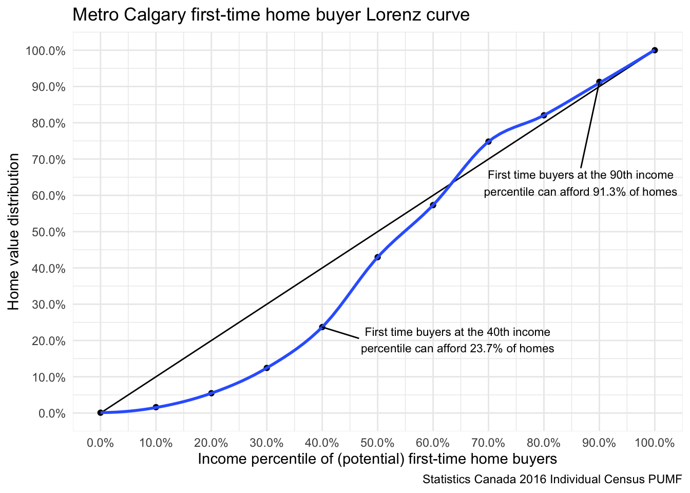
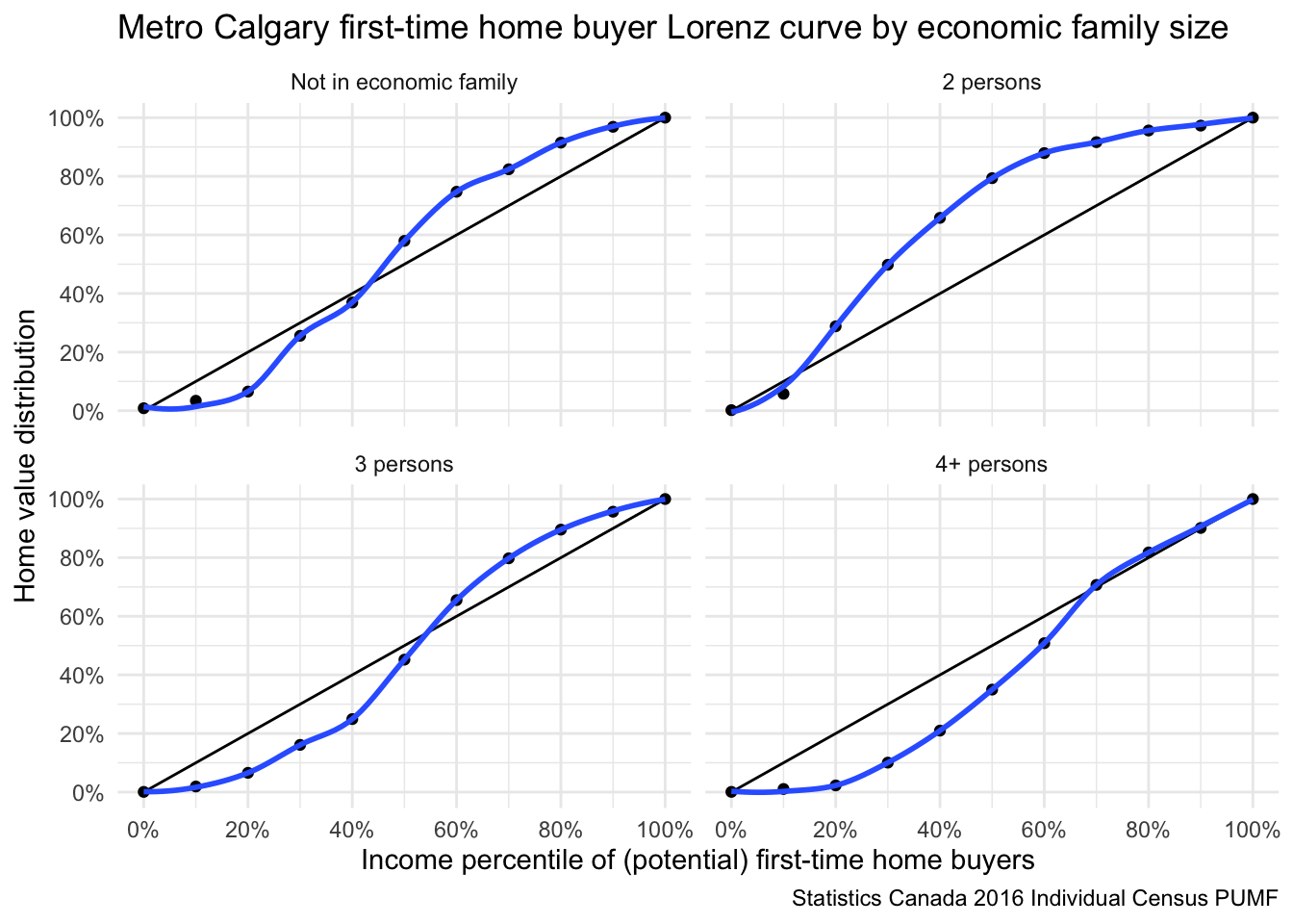
In Calgary, potential first-time buyers at the bottom end of the renter income can’t afford any of the homes. Someone at the 20th income percentile of potential first-time buyers can only afford 5% of Calgary homes. But after that things pick up fast and someone at the 60th percentile can afford 57%, at which point things even out and the Lorenz curve hugs the diagonal.

This says nothing about what kind of home someone can afford, or where in the metro area an affordable home may be, or how well e.g. the number of bedrooms in the home matches the requirements of the potential first-time buyers. It also skirts the discussion about “starter homes” or more generally the question if there is a mismatch between homes first-time buyers are buying and the overall distribution of homes in the metro area in terms of quality or size. Or if there should be such a distinction. What this does is it gives a rough matchup between incomes of (potential) first-time buyers and home values.

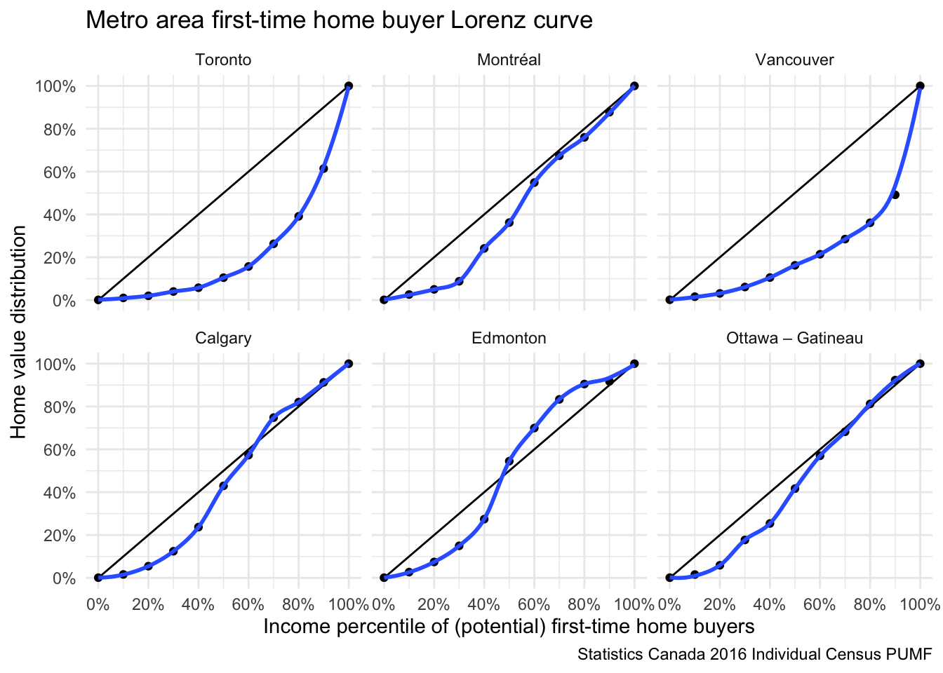
Looking at the Calgary data we are led to ask if the Calgary Lorenz curve is typical for Canadian metropolitan areas. Looking at the largest six metro areas, the answer is mostly Yes, except for Toronto and Vancouver.

Note: The Census Public Use Micro File (PUMF) combines smaller metropolitan areas in the same province together (e.g. Regina-Saskatoon).

Looking more broadly, Victoria and Hamilton have patterns broadly similar to Toronto and Vancouver, with Oshawa also exhibiting a lot of similarities, except in the top income decile.

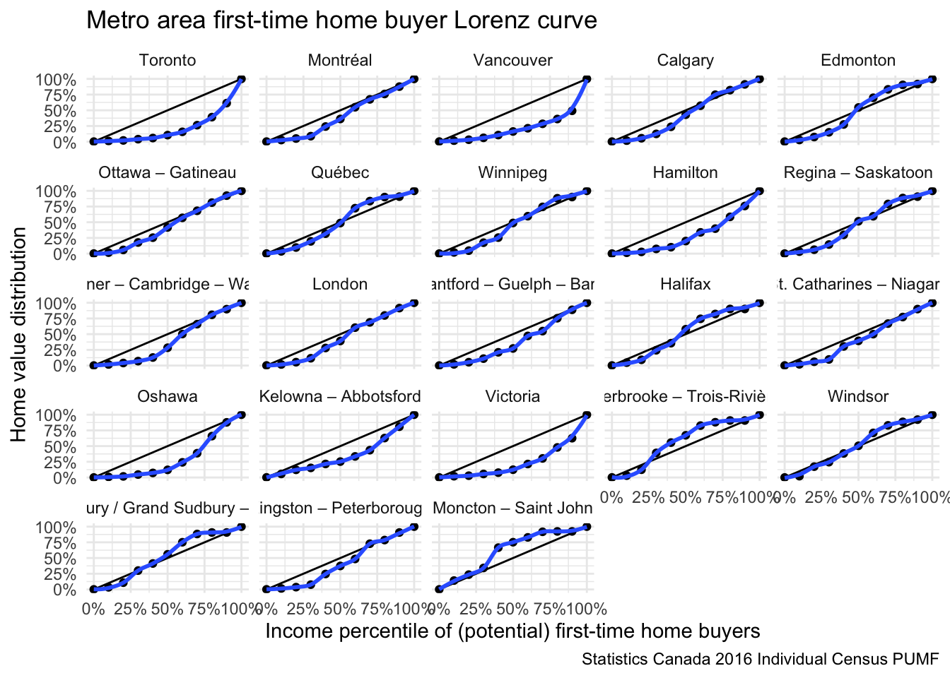
This begs several questions: * Is there a good way to condense these graphs into a simple to use metric? * How does such a metric compare to median multiples? * What are ways that we can refine the Lorenz curves to account for needed space and not just affordability?

The first times buyer GINI index

The term “Lorenz curve” that we have adapted from Meen and Whitehead is a bit of a misnomer, Lorenz curves are used to compare a distribution with it’s cdf, we are comparing the cdfs of two different distributions and compare them to a hypothetical case where both match up. One important difference is that our “Lorenz curves” can take values above the diagonal.

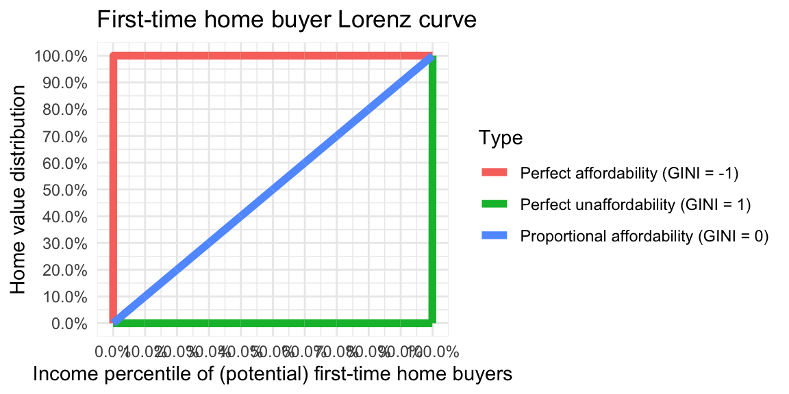
There are many ways to condense the comparison between two distributions into an index, we have recently looked in detail at several such indices. In this case we can stick with our Lorenz curve analogy and compute a First-Time Buyer GINI Index, defined as (double) the (signed) area between the first-time buyer Lorenz curve and the diagonal in analogy to the definition of the regular GINI index The regular GINI index takes values between 0 and 1, our first-time buyer GINI index takes values between -1 and 1. A value of -1 would mean that all potential first-time buyers could afford all homes, a value of 1 corresponds to no buyers being able to afford any of the homes. A value of 0 corresponds to the situation where, on average, a buyer at income percentile \(x\) can buy all homes below the home value percentile \(x\).

Taking the first-time buyer Lorenz curve to be piecewise linear, the calculation of the corresponding GINI coefficient is straight-forward. We contrast the first-time buyer GINI index with the familiar median multiple metric, computed over incomes of all households vs the values of owner-occupied homes.

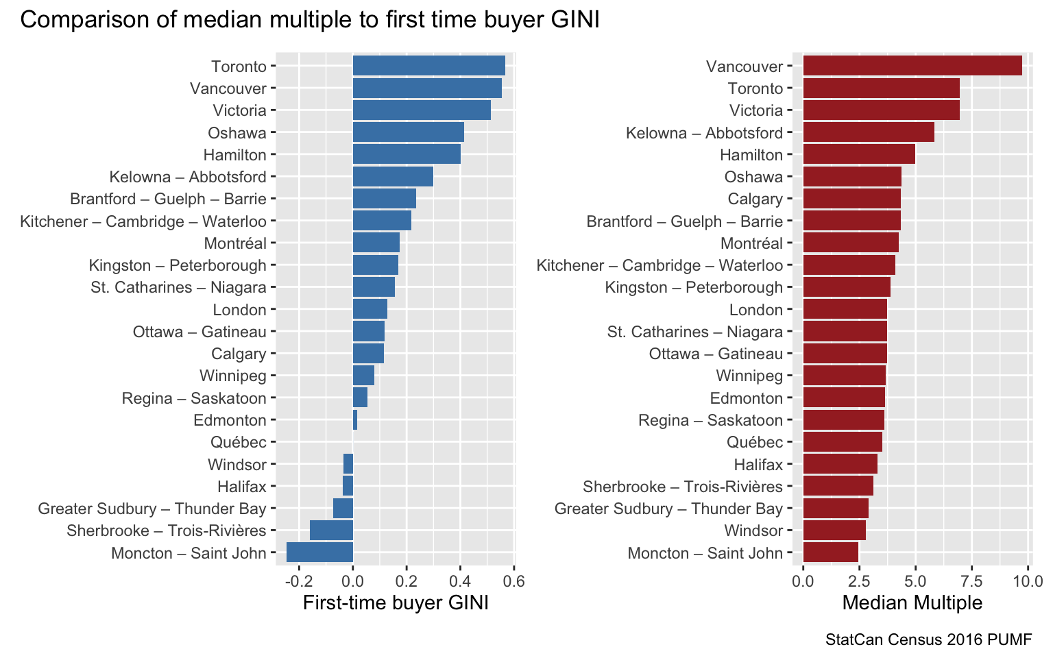
There is a broad correspondence between the two metrics, but it’s interesting to explore the differences. Vancouver as expected stands out on the median multiples chart, but it trades places with Toronto when looking at the first-time buyer GINI index.

Refining the Lorenz curves

One way to refine this is to take a closer look at home size requirements. A one-person household has very different requirements from a 3 or 4 person family. Moreover, household income is probably not the best metric here. Household income is useful when looking at ability to pay shelter costs at the current home, but it is less useful for looking at affordability of buying a new home. Households generally don’t buy homes, family units and unattached individuals do. Economic family income (or maybe census family income) and income of unattached individuals is a better metric to use. And we should match up the family size with the number of bedrooms in a home. After all, we are not that concerned about whether an individual is or is not able to purchase a 4 bedroom home, but we are much more concerned about the ability to purchase a studio or 1-bedroom home. Similarly, it’s not that relevant if a family of 3 can purchase a 1-bedroom unit, but it is very relevant if they can purchase a 2 or 3 bedroom unit.

So we need to make a decision of housing that’s adequate for an economic family, but also does not compare they to homes where they would be “overhoused”. That’s a tricky thing to do, we are going with the following rough categories:

Family size	Number of bedrooms
Single	0 or 1
2 persons	1 or 2
3 persons	2 or 3
4+ persons	3 or more

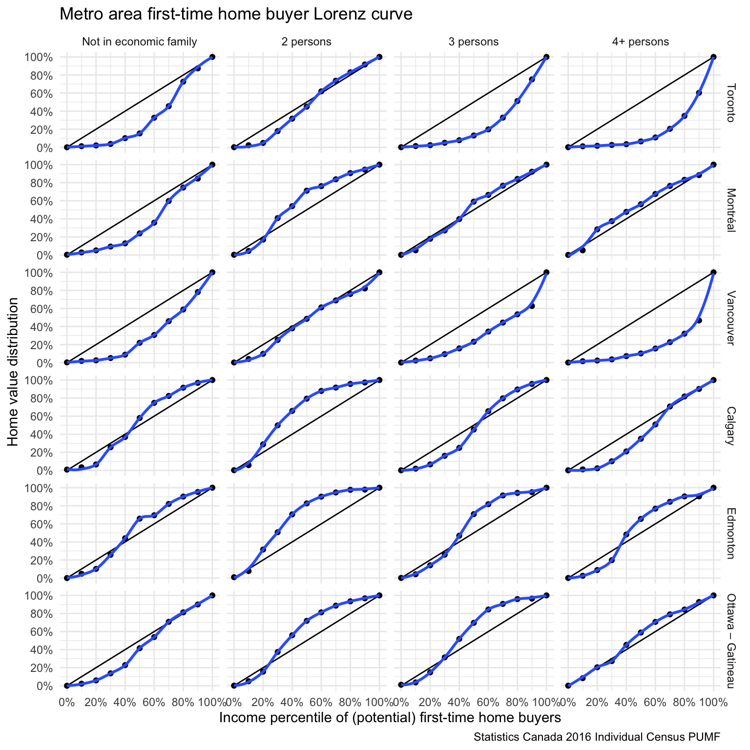
Looking at the distributions we notice that 2 person families fair quite well in terms of this metric.

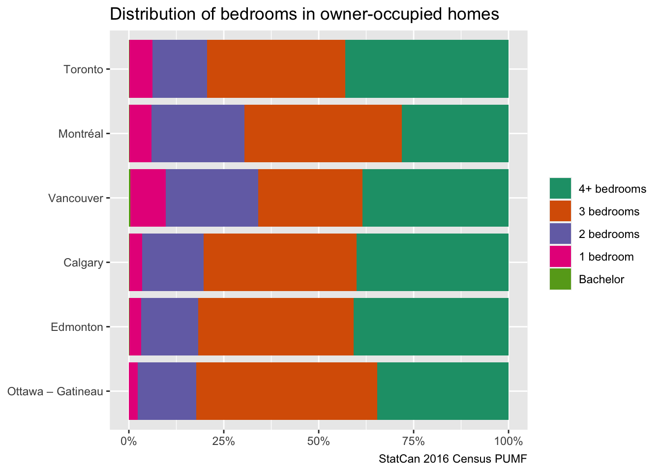
Vancouver and Montreal stand out with a fairly high share of (owner-occupied) 1 and 2 bedroom homes. Montreal also has a noticeably lower share of 4+ bedroom homes, with Ottawa-Gatineau also showing markedly lower levels.

Adjusted first-time buyer GINI index

Dealing with a slew of different family sizes and bedroom counts gets complicated fast, to simplify things we can try and condense the home value into an “adjusted home value”. For our purposes the question is how home values scale with the number of bedrooms. Experimenting with the functional form it appears that dividing by the square root of the number of bedrooms gives a decent fit to normalize the home values. This dove-tails well with the established concept of adjusted family income, that scales family income by the square root of the family size. As an aside, we note that while the adjusted family income is likely a useful metric to measure housing affordability from the perspective of a family, banks and government regulation generally don’t take family size into consideration in loan underwriting requirements.

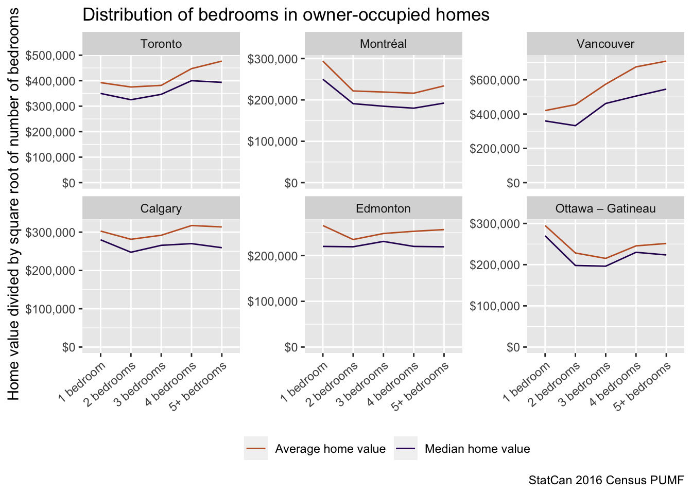
We removed bachelor units from this consideration because there are only very few owner-occupied bachelor units in each CMA. The relationship is nothing to write home about, but good enough for this post. It would be worthwhile to investigate this in more detail. But this likely requires better data, in particular on location as well as better data on dwelling type, which we are missing when working with CMA-level data. Assessment data should work reasonably well for this, but comparable data is not available on a national scale. Ideally we would build our own model, like our (highly experimental and gpu-intensive) interactive fine-geography home valuation model.

For now we will go with the simplistic adjusted home value that divides by the square root of the number of bedrooms, and pair that up with adjusted family income. A choice has to be made for how we should match up people and with homes. We can stick with family units, and homes, or take it down to people and bedrooms. Conceptually it might be easier to work with family units and homes, as this is the level at which purchase decisions are made. The difference when taking it down to people and bedrooms is that families with a larger number of members get weighted more, which seems like a reasonable adjustment. For this post we will stick with matching family units to homes.

Note that this is a little more generous as our previous matchup of bedrooms to families as it implicitly affords each family member their own bedroom, instead of drawing from the distribution of homes with the same or one fewer bedrooms as family members.

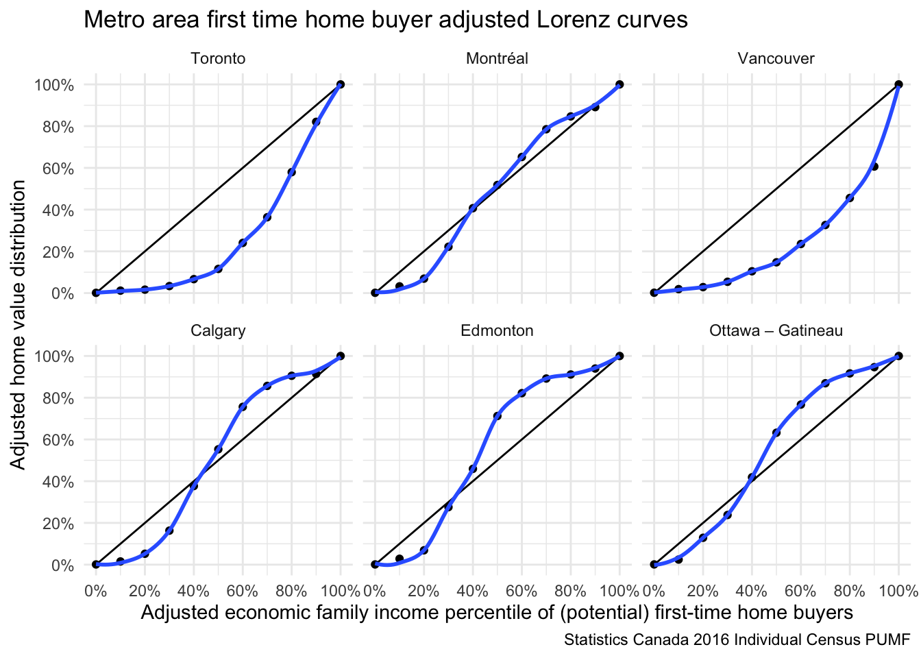
These curves look broadly similar to the ones we had initially by just naively using household income, but taking a closer look we also notice differences, especially at the upper end. We can again condense the data into an adjusted first-time buyer GINI index.

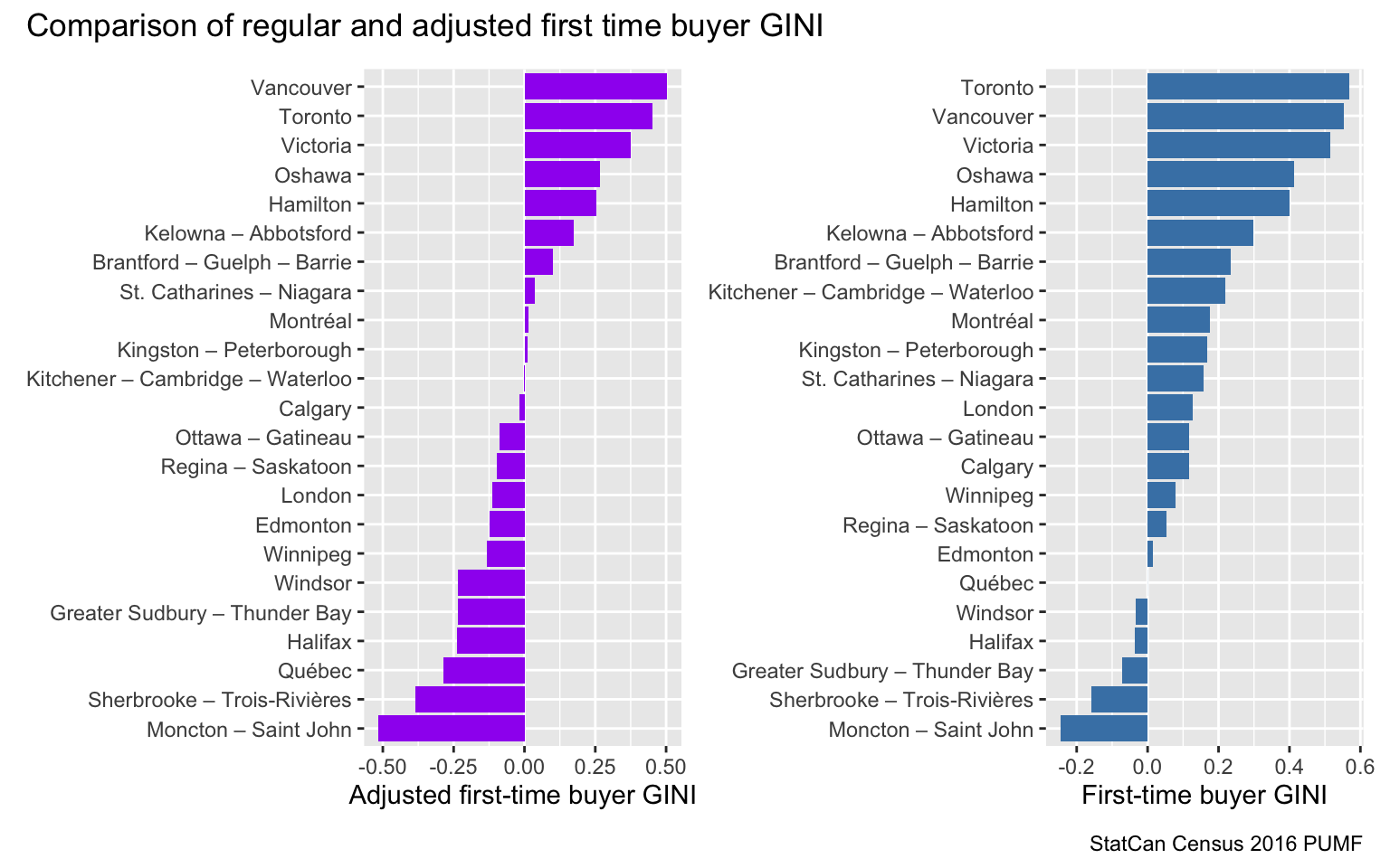
This has the net effect of making housing more affordable for first-time buyers (And shuffles the order a little.) This suggests that one could make substantial affordability gains for first-time buyers by allowing housing to be used, and sold, more flexibly. In Vancouver we already have an important example of that with a comparatively high proliferation of secondary suites, sometimes officially sanctioned but mostly as informal housing. While this helps housing to be used more flexibly, it does little to help with first-time home buyer affordability as this is lacking flexibility on how portions of the house can be sold. Easing restrictions on flexible use of housing, in particular removing the legally dubious municipal definitions of “family” that regulate how a dwelling unit can be shared, as well as adding flexibility in subdividing homes and bringing informal dwelling units into the official housing stock and allowing these to be sold separately, is likely to enhance first-time home buyer affordability. Splitting or combining strata units remains a formidable undertaking in Canada and is rare, this may be an area where Canada can learn from other countries where this is more common.

We should emphasize that having a negative GINI coefficient does not mean that everyone can afford a home matching their position in the income distribution. This is only true on average, as comparing with the Lorenz curve of e.g. Edmonton shows. Condensing the data into an index loses information, and we might want to also retain more complex representations like the Lorenz curve for better context.

Upshot

In summary, Lorenz curves and the derived GINI index provide an interesting view into affordability for first-time buyers, a group whose position has been substantially weakened by growing wealth inequality combined with low interest and property tax rates. We think this provides a useful metric to watch.

Refinements, like the adjusted first-time buyer Lorenz curves and GINI index can help remove distributional effects while still being easy to work with. It would be worthwhile to explore this further, and find a better way to add location information. This may also help firm up the best functional form of the adjustment on home values by bedrooms.

As usual, the code for this post is available on GitHub for anyone to reproduce or adapt for their own purposes.

from Hacker News https://ift.tt/343WewE