Faster-XML Jackson-databind (excludes most polymorphic typing gadget attacks) (Publicly disclosed vulnerability) is used by IBM Operations Analytics Predictive Insights. IBM Operations Analytics Predictive Insights has addressed the applicable CVEs. Note that the usage of Jackson-databind within IBM Operations Analytics Predictive Insights is limited to the REST Mediation utility. If you do not have this service installed you are not affected by this bulletin.
There are multiple vulnerabilities in IBM® Java™ SDK Technology Edition, Oct 2019 used by IBM Security Identity Manager Virtual Appliance. IBM Security Identity Manager Virtual Appliance has addressed the applicable CVEs.
Faster-XML Jackson is used by IBM Operations Analytics Predictive Insights. IBM Operations Analytics Predictive Insights has addressed the applicable CVEs. Note that the usage of Jackson Databind within IBM Operations Analytics Predictive Insights is limited to the REST Mediation utility. If you do not have this utility installed you are not affected by this bulletin, otherwise apply the recommended remediation fixes.
Apache Thrift is vulnerable to a denial of service, caused by an error when processing untrusted Thrift payload. A remote attacker could exploit this vulnerability to cause the application to enter into an infinite loop.
Websphere Application Server (Liberty profile) is shipped as a component of IBM Operations Analytics Predictive Insights. Information about a security vulnerability affecting Liberty profile has been disclosed in a security bulletin.
There is a spoofing vulnerability in the IBM HTTP Server used by WebSphere Application Server version 9. This vulnerability has been fixed in IBM HTTP Server version 9.0.0.3.
Affected product(s) and affected version(s):
This vulnerability affects the following version and release of IBM HTTP Server (powered by Apache) component in all editions of WebSphere Application Server and bundling products.
Jackson s used by IBM Operations Analytics Predictive Insights. IBM Operations Analytics Predictive Insights has addressed the applicable CVEs. Note that the usage of Jackson Databind within IBM Operations Analytics Predictive Insights is limited to the REST Mediation utility. If you do not have this utility installed you are not affected by this bulletin, otherwise apply the recommended remediation fixes.
There are multiple vulnerabilities in IBM® SDK Java™ Technology Edition, Version 7.0.10.50 used by IBM Cloud Manager with OpenStack. These issues were disclosed as part of the IBM Java SDK updates in April 2020.
jackson-databind (excludes most polymorphic typing gadget attacks) is used by IBM Operations Analytics Predictive Insights. IBM Operations Analytics Predictive Insights has addressed the applicable CVEs. Note that the usage of Jackson Databind within IBM Operations Analytics Predictive Insights is limited to the REST Mediation utility. If you do not have this utility installed you are not affected by this bulletin, otherwise apply the recommended remediation fixes.
Faster-XML Jackson-databind is used by IBM Operations Analytics Predictive Insights. IBM Operations Analytics Predictive Insights has addressed the applicable CVEs. Note that the usage of Jackson Databind within IBM Operations Analytics Predictive Insights is limited to the REST Mediation utility. If you do not have this utility installed you are not affected by this bulletin, otherwise apply the recommened remediation fixes.
Australia is drafting a new regulation that misunderstands the dynamics of the internet and will do damage to the very news organisations the government is trying to protect. When crafting this new legislation, the commission overseeing the process ignored important facts, most critically the relationship between the news media and social media and which one benefits most from the other.
Assuming this draft code becomes law, we will reluctantly stop allowing publishers and people in Australia from sharing local and international news on Facebook and Instagram. This is not our first choice – it is our last. But it is the only way to protect against an outcome that defies logic and will hurt, not help, the long-term vibrancy of Australia’s news and media sector.
We share the Australian Government’s goal of supporting struggling news organisations, particularly local newspapers, and have engaged extensively with the Australian Competition and Consumer Commission that has led the effort. But its solution is counterproductive to that goal. The proposed law is unprecedented in its reach and seeks to regulate every aspect of how tech companies do business with news publishers. Most perplexing, it would force Facebook to pay news organisations for content that the publishers voluntarily place on our platforms and at a price that ignores the financial value we bring publishers.
The ACCC presumes that Facebook benefits most in its relationship with publishers, when in fact the reverse is true.News represents a fraction of what people see in their News Feed and is not a significant source of revenue for us. Still, we recognize that news provides a vitally important role in society and democracy, which is whywe offer free tools and training to help media companies reach an audience many times larger than they have previously.
News organisations in Australia and elsewhere choose to post news on Facebook for this precise reason, and they encourage readers to share news across social platforms to increase readership of their stories. This in turn allows them to sell more subscriptions and advertising. Over the first five months of 2020 we sent 2.3 billion clicks from Facebook’s News Feed back to Australian news websites at no charge – additional traffic worth an estimated $200 million AUD to Australian publishers.
We already invest millions of dollars in Australian news businesses and, during discussions over this legislation, we offered to invest millions more. We had also hoped to bringFacebook Newsto Australia,a feature on our platform exclusively for news, where we pay publishers for their content. Since it launched last year in the US, publishers we partner with have seen the benefit of additional traffic and new audiences.
But these proposals were overlooked.Instead, we are left with a choice of either removing news entirely or accepting a system that lets publishers charge us for as much content as they want at a price with no clear limits. Unfortunately, no business can operate that way.
Facebook products and services in Australia that allow family and friends to connect will not be impacted by this decision. Our global commitment to quality news around the world will not change either. And we will continue to work with governments and regulators who rightly hold our feet to the fire. But successful regulation, like the best journalism, will be grounded in and built on facts. In this instance, it is not.
Read more about Facebook’s response to Australia’s News Media and Digital Platforms Mandatory Bargaining proposed legislation.
A History of U.S. Foreign Policy from Z to Shining Z
In this episode of Horns of a Dilemma, William Inboden, editor-in-chief of the Texas National Security Review, is joined by Robert Zoellick, former president of the World Bank, and Philip Zelikow, former executive director of the 9/11 Commission and counselor to numerous administrations, to discuss Zoellick’s new book, America in the World: A History of U.S. Diplomacy and Foreign Policy. They also discuss how Zoellick transformed himself from an economist, an expert in finance, a lawyer, and a diplomat, into a historian who wrote an overarching history of a vast period of American power.
I am an infectious disease doctor and a professor of medicine at the University of California, San Francisco. As governments and workplaces began to recommend or mandate mask wearing, my colleagues and I noticed an interesting trend. In places where most people wore masks, those who did get infected seemed dramatically less likely to get severely ill compared to places with less mask-wearing.
No mask is perfect, and wearing one might not prevent you from getting infected. But it might be the difference between a case of COVID-19 that sends you to the hospital and a case so mild you don’t even realize you’re infected.
The higher the viral dose, the higher the chance of developing severe COVID-19 that could require hospitalization.AP Photo/Kathy Willens
Exposure dose determines severity of disease
When you breathe in a respiratory virus, it immediately begins hijacking any cells it lands near to turn them into virus production machines. The immune system tries to stop this process to halt the spread of the virus.
The amount of virus that you’re exposed to – called the viral inoculum, or dose – has a lot to do with how sick you get. If the exposure dose is very high, the immune response can become overwhelmed. Between the virus taking over huge numbers of cells and the immune system’s drastic efforts to contain the infection, a lot of damage is done to the body and a person can become very sick.
On the other hand, if the initial dose of the virus is small, the immune system is able to contain the virus with less drastic measures. If this happens, the person experiences fewer symptoms, if any.
This concept of viral dose being related to disease severity has been around for almost a century. Many animal studies have shown that the higher the dose of a virus you give an animal, the more sick it becomes. In 2015, researchers tested this concept in human volunteers using a nonlethal flu virus and found the same result. The higher the flu virus dose given to the volunteers, the sicker they became.
In July, researchers published a paper showing that viral dose was related to disease severity in hamsters exposed to the coronavirus. Hamsters who were given a higher viral dose got more sick than hamsters given a lower dose.
Based on this body of research, it seems very likely that if you are exposed to SARS-CoV-2, the lower the dose, the less sick you will get.
So what can a person do to lower the exposure dose?
Most infectious disease researchers and epidemiologists believe that the coronavirus is mostly spread by airborne droplets and, to a lesser extent, tiny aerosols. Research shows that both cloth and surgical masks can block the majority of particles that could contain SARS-CoV-2. While no mask is perfect, the goal is not to block all of the virus, but simply reduce the amount that you might inhale. Almost any mask will successfully block some amount.
The final piece of experimental evidence showing that masks reduce viral dose comes from another hamster experiment. Hamsters were divided into an unmasked group and a masked group by placing surgical mask material over the pipes that brought air into the cages of the masked group. Hamsters infected with the coronavirus were placed in cages next to the masked and unmasked hamsters, and air was pumped from the infected cages into the cages with uninfected hamsters.
As expected, the masked hamsters were less likely to get infected with COVID-19. But when some of the masked hamsters did get infected, they had more mild disease than the unmasked hamsters.
Every passenger aboard the Greg Mortimer, a cruise ship bound for Antarctica, was given a surgical face mask.AP Photo/Matilde Campodonico
However, in places where everyone wears masks, the rate of asymptomatic infection seems to be much higher. In an outbreak on an Australian cruise ship called the Greg Mortimer in late March, the passengers were all given surgical masks and the staff were given N95 masks after the first case of COVID-19 was identified. Mask usage was apparently very high, and even though 128 of the 217 passengers and staff eventually tested positive for the coronavirus, 81% of the infected people remained asymptomatic.
There is no doubt that universal mask wearing slows the spread of the coronavirus. My colleagues and I believe that evidence from laboratory experiments, case studies like the cruise ship and food processing plant outbreaks and long-known biological principles make a strong case that masks protect the wearer too.
The goal of any tool to fight this pandemic is to slow the spread of the virus and save lives. Universal masking will do both.
The story of the werewolf is perhaps the most famous anecdote from Petronius’ Satyricon, a staple of Latin literature written in the first century. In the tale, a guest at a dinner party offers a marvelous tale of transformation and mystery. A Roman slave and a houseguest rush off into the night. In a cemetery shrouded by ethereal moonlight, one of them is delivered of his human form and given new life as a ferocious beast.
In addition to its absurdity, the werewolf episode is special for its language. In the entirety of Latin literature, the only known usage of the word “apoculamus” (“we rush off”) is in section 62 of the Satyricon. As a result, this verb is considered a hapax legomenon, a word that occurs only once in a text, an author’s oeuvre, or a language’s entire written record.
The Satyricon contains a number of hapaxes, including “bacalusias” (possibly “sweetmeat” or ”lullabies”) and “baccibalum” (“attractive woman”).
Hapaxes are not limited to Latin. They appear in every language, from Arabic to Icelandic, even English. But where do these words come from, and what is their purpose?
Various theories have been posited about the role of hapaxes. In a 1955 lecture, philologist Joshua Whatmough suggested that the poet Catullus inserted them to draw attention to a specific moment, just as poet Ezra Pound would do centuries later. Others hold that authors do not pay attention to the frequency of specific languages in their writing, suggesting that words become hapaxes only by chance.
There are various methods applied to translate hapaxes that aren’t conventional words. In the case of “apoculamus” from the Satyricon, classicists can use context and precedent to define the term. At this point in the story, the narrator is describing how he and his companion departed from their house. From the ending “-mus,” we know that this word is a first-person plural, present, active, indicative verb. Therefore, “apoculamus” can be interpreted as a form of movement.
Given the influence of ancient Greek on Latin, scholars have also relied on etymology for translation hints. The prefix “apo” means “away from” and the noun “culum” refers to a person’s buttocks. Hence, “apoculamus” might be defined as “hauling your posterior away from” something.
Petronius Arbiter, author of Satyricon. Public Domain
Some scholars disagree with these suggestions, arguing that “apoculamus” was not in the original text. The Satyricon has come to us in fragments, which means that the language might not be accurate to the original version. Therefore, it is possible that Petronius used a different verb, which was miscopied by a scribe at some point. Like the game of telephone, the most recent copy of the novel may have been altered from its initial form, prompting scholars to question the correctness of “apoculamus.”
There are a number of words from classical Greek and Latin that we will never be able to translate with certainty. One that has stumped scholars is “πολεμοφθόροισιν” (“polemophthoroisin”), which can be found in line 653 of Aeschylus’ The Persians, a Greek tragedy written in the fifth century B.C. The play narrates the return of the Persian king Xerxes from Greece, following his disastrous defeat at the Battle of Salamis. In this scene, the chorus is praising the former king, Darius, who is remembered as a just ruler for not “prompting the downfall of his men through meaningless wars,” as opposed to his son. Based on context of the section, classicists assume that the term relates to war in some way. “πόλεμος” (“Polemos”) was, for the Greeks, the divine personification of battle, while “φθείρω” (“ftheiro”) translates as “destroy.” Hence, the combination of the two might mean “destruction by war,” which is what Xerxes has done by attacking the Greeks.
An illustration of a scene in Aeschylus’ The Persians, which includes the difficult-to-translate word πολεμοφθόροισιν—“polemophthoroisin.” Public Domain
Catullus, a poet who wrote in Latin during the first century B.C., used hapaxes often, “ploxeni” in Poem 97 being an especially notable example. The word is of Gaulish origin and refers to a “manure wagon,” a term put to perfect use in this invective against a man named Aemilius. The poem is a virulent attack on his appearance and malodor. Catullus describes Aemilius’ gums as “looking like a manure wagon” on account of their filth. The term “ploxenum” was not used in any other poems, likely due to its obscure derivation.
In Homer’s Iliad, written around the eighth century B.C., we find a hapax in book 2, line 217. The poem chronicles the epic battle between the Greeks and Trojans after the Spartan king Menelaus’ wife, Helen, was abducted by Prince Paris of Troy. Odysseus, the craftiest soldier in the army, is inciting the Greek troops to arms with an stimulating oration. However, he is interrupted by Thersites, a man described as unattractive and odious. Though he is characterized in only a brief passage, Thersites receives the harshest of words: “evil-favored” with “disorderly thoughts” and “rounded shoulders.” The term “φολκός” is among these details. This hapax has been translated as “bow-legged,” an apparent blow to Thersites’ honor.
One of the most famous Shakespearean hapaxes is “honorificabilitudinitatibus,” meaning “able to achieve honors.” The word appears only in Act V, Scene 1 of Love’s Labour’s Lost and is the dative form of a medieval Latin word, “honorificabilitudinitas.” After Shakespeare, authors such as James Joyce and Charles Dickens incorporated it into their works as well.
It is estimated that there are thousands of hapaxes in the Bible. Greek and Latin literature allow us to translate many of the terms from the Septuagint or the Vulgate, the Koine Greek Old Testament and the Latin Bible, respectively. However, since the Old Testament is almost all we have of the ancient Hebrew language, hapaxes can be restrictive. The Song of Songs, which is the last section of the Tanakh and part of the Christian Old Testament, contains an especially high number of hapax legomena, forcing scholars to rely on the Greek version for translation hints. The Song of Songs is, at the surface, a story of love between a man and a woman, in which they describe their passion for each other. It has the greatest number of hapaxes in the Bible, rendering the book enigmatic and mysterious. For instance, in 4.13, the male compares the lady’s “selahim” to an orchard. The term is a hapax, but scholars have suggested “branches” as a translation, such that the text describes the woman’s body.
A linguistic phenomenon similar to hapaxes is the nonce word. Authors can, in effect, produce hapaxes by creating words. Shakespeare is famous for his frequent usage of such terms. In the Taming of the Shrew, a play about matrimony and courtship, the main character Katherina, describes herself as being “bedazzled” by the sun. This word was coined by the bard for this scene, but has now received commercial fame courtesy of a rhinestoning device.
Despite the uncertainty that comes with hapaxes, one thing is clear: these words form an intriguing linguistic phenomenon, one which we may never be able to solve.
There's a long and painful discussion on the setuptools issues
list (I count 9 issues raised the day after the release). This is all
to do with how Debian/Ubuntu installs stuff with pip.

There's an "official" workaround that involves setting things in your
environment, but that looks a bit fiddly with the Azure pipelines
stuff and this has been such a disaster that I'm pretty certain the
setuptools maintainers will release something more sensible soon.

See e.g.
pypa/setuptools#2350 (comment)
for a careful description of what's going on.

Signed-off-by: Rupert Swarbrick <rswarbrick@lowrisc.org>
- Added setuptools 49.1.0 to hopefully resolve new issue with loading hug libraries on ubuntu/debian (lambada run-times)
- See: pypa/setuptools#2232 and pypa/setuptools#2350

Signed-off-by: David Deal <dealako@gmail.com>
Converting Boolean-Logic Decision Trees to Finite State Machines
for simpler, high-performance detection of cybersecurity events
When analyzing cybersecurity events, the detection algorithm evaluates attributes against boolean expressions to determine whether the event belongs to a class. This article describes converting boolean expressions to finite state machines to permit simpler, high-performance evaluation.
The open-source project Cyberprobe features this implementation. Conversion of rules to finite state machine (FSM) and application of the rules in FSM form is implemented in Python. Cyberprobe supports the use of millions of rules, which can be applied at greater than 200k events/second on a single processor core.
Problem
Applying boolean logic criteria to events solves many scanning and detection problems. For instance, an event occurs that is generated from an interaction with a service under protection. The event has the following attributes:
Source address: 123.123.123.123:14001
Destination address: 192.168.0.1:19001
URL: https://myservice.com/path1
One or more boolean expressions for the class of thing I am trying to detect:
If TCP port number is 80 or 8080 AND IP address is 10.0.0.1 AND URL is https://ift.tt/3hMmj8Y OR https://ift.tt/2YR7BWO …
The aim is to analyze a high-rate stream of such events against a large set of boolean expressions to classify the events.
The boolean expressions get unreadable quickly with English, which has no built-in operator precedence.
Boolean expressions
Boolean operators are represented as functions, and type:value represents attribute type/value match terms.
A boolean expression consists of a combination of, and(…), or(…) and not(…) functions, along with type:value match terms. I am using type:value pairs for match terms as that is useful in the domain I’m working in, but we could just as easily use strings.
Input
When evaluating the attributes of an event, attributes are type:value pairs. e.g.
A simple approach for evaluation of a boolean expression using type:value pair input is to represent the boolean expression as a tree, and then use type:value pairs to trigger evaluation. Observations are stored in the tree.
The rules for evaluating a boolean tree against an event are:
For each type:value attribute, see if there is a corresponding type:value term in the boolean tree. If it exists, set the term node as true, and evaluate the parent node.
When evaluating a parent or node, when any child is true, the or node is true, and its parent node is evaluated.
When evaluating a parent and node, when ALL children are true, the and node is true, and its parent node is evaluated.
When evaluating a parent not node, when the child node is true, the not node is false. Once evaluation of all attributes is complete, if a not node has not been deemed false because its child is false, then it is evaluated true, and it’s parent node is evaluated.
That’s a straightforward algorithm; the point of this article is to provide an optimization.
There is a compromise here, the algorithm to convert the boolean tree to an FSM is compute intensive: it has complexity which is non-linear with the number of nodes: it is linear with the product of combination nodes (described below) and type:value terms. In real-world scenarios, boolean expressions will be converted to FSM when the rule is parsed, thereafter the FSM can be used numerous times.
Converting to an FSM
Step 1: Identify the ‘basic states’
In order to find the FSM, we look for all of the nodes in the boolean tree where state needs to be observed as evaluation proceeds. If you look at the example above, you can see that or nodes and and nodes are different. A child of an or node when evaluated as true immediately results in its parent being true, so no state needs to be kept regarding the children of or nodes. Whereas, when a child of an and node is true this is something which may need to be stored for later evaluation to determine the point at which the and node can be evaluated true.
The evaluation of not nodes is also complicated: a not node can be evaluated as true by virtue of its child maintaining a false evaluation for the duration of analysis.
The rules we state here are that some nodes in the boolean tree can be described as basic states:
The root of a tree is inherently a hit state, which means the boolean expression is true. This is a basic state.
A not node is never a basic state.
A child of an and node is a basic state unless it is a not node.
A child of a not node is a basic state unless it is a not node itself.
In the above example, the basic states are the two or nodes, and the ip:10.0.0.1 node. All qualify under rule 3.
The implementation gives each state a state name which consists of the letter s plus a unique number, assigned in a depth-first walk. The example boolean tree with states is shown below; the three children of the and node are given states, with the parent and node representing the hit state.
Step 2: Identify the ‘combination states’
The basic states are nodes where partial state needs to be recorded. One node in an FSM represents all state at the same time i.e. all the valid basic state combinations. Hence the combination states set consists all combinations of basic states. This includes the empty set, and a union of all states.
Combination states need to have a state name: in my implementation, I combine states to a name by ordering, separating state numbers with a hyphen preceded by s. For example, a combination of states s4, s7, s13 is called s4–7-13.
The empty set has a special name which we call init. It represents the initial state of the FSM where no information is known.
There is a special state hit which is used to describe any combination of basic states which include the root node evaluating to true. The combination of other states is ignored.
In the above example, the combination state set consists of:
init: The empty set
s3: The first or node:
s4: The ip:10.0.0.1 node
s7: The second or node
s3-4: The first or node and ip:10.0.0.1
s4-7: The ip:10.0.0.1 node and the second or node
s3-7: The first and second or nodes
hit: the root node
Step 3: Find all match terms
This is the set of all type:value match nodes in the boolean expression tree.
Step 4: Find all transitions
This step is essentially about working out what all type:value match nodes do to all combination states. There is a special match term, end: which is used to evaluate what happens to not nodes when the list of terms is completed.
The algorithm is:
For every combination state:
    Work out the state name of that 'input' combination state
    For every match term:
        Given the input state
        What state results from evaluating that term as true?
        Work out the state name of that 'output' combination state
        Record a transition (input, match term, output)
    Given the input state
    What state results from evaluating end: as true?
    Work out the state name of that 'output' combination state
    Record a transition (input, end:, output)
For this analysis, when the whole boolean expression evaluates as true i.e. the root node of the boolean expression is true, we give that a special name hit.
The result is a complete set of triples: (input, term, output). If the input and output states are the same, we can ignore the transition so that the FSM only contains edges which change state.
At this point, the FSM has some inefficiencies: there may be areas of the FSM which it is not possible to navigate to from init. This is addressed in the next step.
Step 5: Remove invalid transitions
Not all combination states can be reached from init, and so some of the transitions discovered can be discarded as irrelevant.
We start by constructing a set of states which can navigate to hit:
Create a set containing only the combination state hit.
Iterate over the FSM adding all transitions for which there is a navigation to any state in the set.
Repeat 2. until the full set of states is discovered.
At this point we know all states which can lead to hit. However, there will be transitions which lead to states which are not in this set, and thus cannot ever travel to hit. So, the first simplification of invalid transitions is to reduce all transitions to states which are NOT in this set to the single state named fail.
There is a second simplification of the FSM: some of the states are not navigable from init, and can be removed:
Construct a set containing only init.
Iterate over the FSM finding all transitions for which there is a navigation from any state in the set.
Repeat 2. until the set of states is discovered.
At this point we know areas of the FSM which are not reachable, and they can be removed.
Resultant FSM
The FSM of the above binary tree is depicted below. The init state represents the initial FSM state. The hit state represents successful evaluation of the boolean expression as true. We have mentioned the fail state, which only occurs when not expressions are used, which do not appear as a result of the boolean expression described as above. See below for an example.
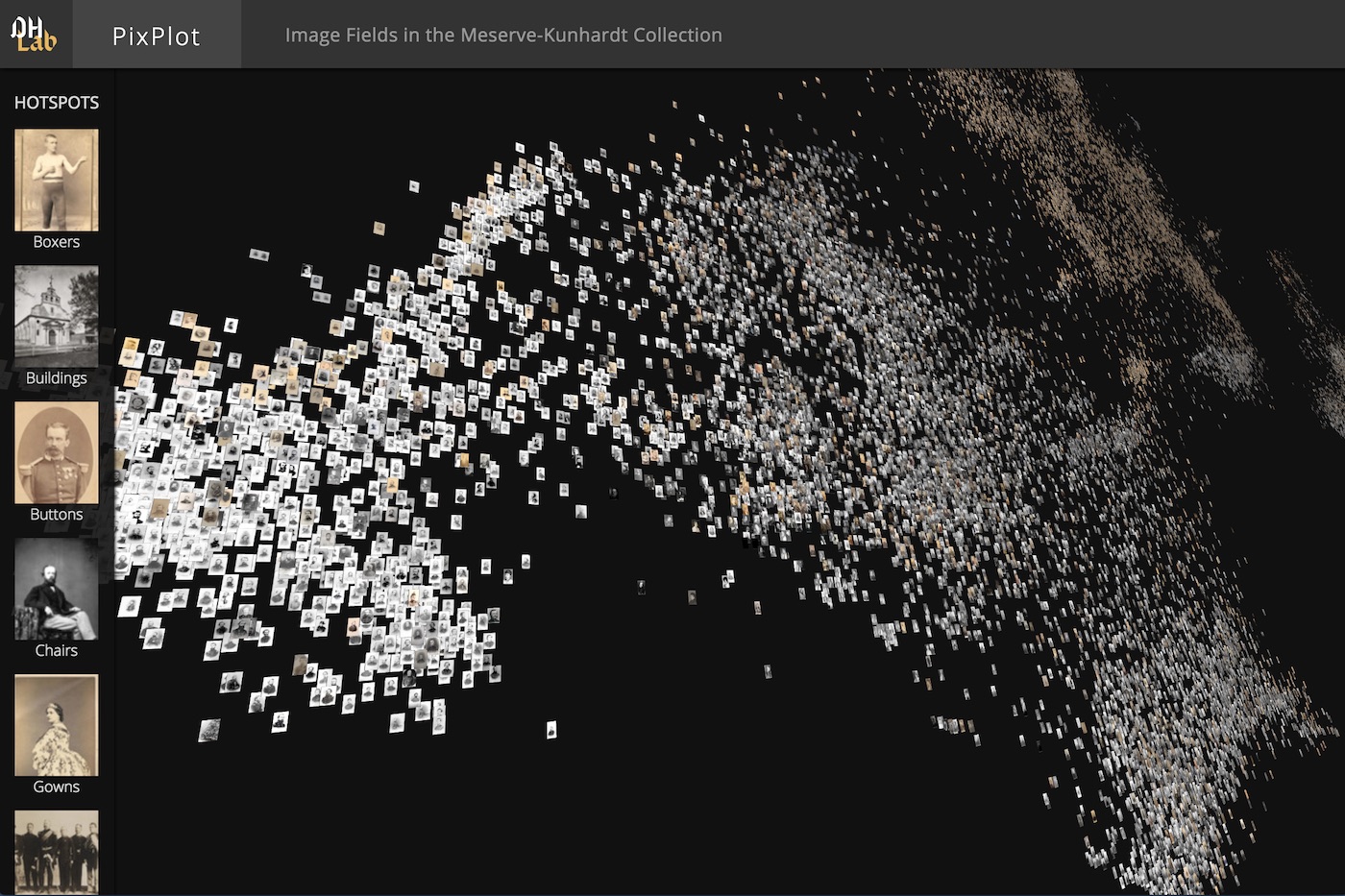
For the last year or so, Yale’s DHLab has undertaken a series of experiments organized around analysis of visual culture. Some of those experiments have involved identifying similar images and visualizing patterns uncovered in this process. In this post, I wanted to discuss how we used the amazing Three.js library to build a WebGL-powered visualization that can display tens of thousands of images in an interactive 3D environment [click to enter]:
If you’re interested in creating something similar, feel free to check out the full code.
Getting Started with Three.js
Three.js is a JavaScript library that generates lower-level code for WebGL, the standard API for 3D rendering in a web browser. Using Three.js, one can build complex 3D environments that would take much more code to build in raw WebGL. For a quick sample of the projects others have built with the library, check out the Three.js homepage.
To get started with Three.js, one needs to provide a bit of boilerplate code with the three essential elements of a Three.js page:
scene: The scene contains all objects to be rendered:
// Create the scene and a camera to view itvarscene=newTHREE.Scene();
camera: The camera determines the position from which viewers see the scene:
// Specify the portion of the scene visiable at any time (in degrees)varfieldOfView=75;// Specify the camera's aspect ratiovaraspectRatio=window.innerWidth/window.innerHeight;// Specify the near and far clipping planes. Only objects// between those planes will be rendered in the scene// (these values help control the number of items rendered// at any given time)varnearPlane=0.1;varfarPlane=1000;// Use the values specified above to create a cameravarcamera=newTHREE.PerspectiveCamera(fieldOfView,aspectRatio,nearPlane,farPlane);// Finally, set the camera's position in the z-dimensioncamera.position.z=5;
renderer: The renderer renders the scene to a canvas element on an HTML page:
// Create the canvas with a renderer and tell the// renderer to clean up jagged aliased linesvarrenderer=newTHREE.WebGLRenderer({antialias:true});// Specify the size of the canvasrenderer.setSize(window.innerWidth,window.innerHeight);// Add the canvas to the DOMdocument.body.appendChild(renderer.domElement);
The code above creates the scene, adds a camera, and renders the canvas to the DOM. Now all we need to do is add some objects to the scene.
Each item rendered in a Three.js scene has a geometry and a material. Geometries use vertices (points) and faces (polygons described by vertices) to define the shape of an object, and materials use textures and colors to define the appearance of that shape. A geometry and a material can be combined into a mesh, which is a fully composed object ready to be added to a scene.
The example below uses the high-level BoxGeometry, which comes with pre-built vertices and faces:
// Create a cube with width, height, and depth set to 1vargeometry=newTHREE.BoxGeometry(1,1,1);// Use a simple material with a specified hex colorvarmaterial=newTHREE.MeshBasicMaterial({color:0xffff00});// Combine the geometry and material into a meshvarcube=newTHREE.Mesh(geometry,material);// Add the mesh to the scenescene.add(cube);
Finally, to render the scene on the page, one must call the render() method, passing in the scene and the camera as arguments:
renderer.render(scene,camera);
Combining the snippets above gives the following result:
This is great, but the scene is static. To add some animation to the scene, one can periodically update the cube’s rotation property, then rerender the scene. To do so, one can replace the renderer.render() line above with a render loop that calls itself recursively. Here is a standard render loop in Three.js:
functionanimate(){requestAnimationFrame(animate);renderer.render(scene,camera);// Rotate the object a bit each animation framecube.rotation.y+=0.01;cube.rotation.z+=0.01;}animate();
Adding this block at the bottom of the script makes the cube slowly rotate:
Adding lights to the scene can make it easier to differentiate the faces of the cube. To add lights to the scene above, we’ll first want to change the cube’s material, because as the documentation says the MeshBasicMaterial is not affected by lights. Let’s replace the material defined above with a MeshPhongMaterial:
Next let’s point a light at the cube so that different faces of the cube catch different amounts of light:
// Add a point light with #fff color, .7 intensity, and 0 distancevarlight=newTHREE.PointLight(0xffffff,.7,0);// Specify the light's position in the x, y, and z dimensionslight.position.set(1,1,100);// Add the light to the scenescene.add(light)
The snippets above give a quick overview of the core elements of a Three.js scene. The following section will build upon those ideas to create a TSNE map of images.
To build an image viewer, we’ll need to load some image files into some Three.js materials. We can do so by using the TextureLoader:
// Create a texture loader so we can load the image filevarloader=newTHREE.TextureLoader();// Specify the path to an imagevarurl='https://s3.amazonaws.com/duhaime/blog/tsne-webgl/assets/cat.jpg';// Load an image file into a MeshLambert materialvarmaterial=newTHREE.MeshLambertMaterial({map:loader.load(url)});
Now that the material is ready, the remaining steps are to generate a geometry from the image, combine the material and geoemtry into a mesh, and add the mesh to the scene, just like the cube example above. Because images are two-dimensional planes, we can use a simple PlaneGeometry for this object’s geometry:
// create a plane geometry for the image with a width of 10// and a height that preserves the image's aspect ratiovargeometry=newTHREE.PlaneGeometry(10,10*.75);// combine the image geometry and material into a meshvarmesh=newTHREE.Mesh(geometry,material);// set the position of the image mesh in the x,y,z dimensionsmesh.position.set(0,0,0)// add the image to the scenescene.add(mesh);
It’s worth noting that one can swap out the PlanarGeometry for other geometries and Three.js will automatically wrap the material over the new geometry. The example below, for instance, swaps the PlanarGeometry for a more interesting Icosahedron geometry, and rotates the icosahedron inside the render loop:
// use an icosahedron geometry instead of the planar geometryvargeometry=newTHREE.IcosahedronGeometry();// spin the icosahedron each animation framefunctionanimate(){requestAnimationFrame(animate);renderer.render(scene,camera);mesh.rotation.x+=0.01;mesh.rotation.y+=0.01;mesh.rotation.z+=0.01;}animate();
The examples above use a few different geometries built into Three.js. Those geometries are based on the fundamental THREE.Geometry class, which is a primitive geometry one can use to create custom geometries. THREE.Geometry is lower-level than the prebuilt geometries used above, but it gives performance gains that make it worth the effort.
Let’s create a custom geometry by calling the THREE.Geometry constructor, which takes no arguments:
vargeometry=newTHREE.Geometry();
This geometry object doesn’t do much yet, because it doesn’t have any vertices with which to ariculate a shape. Let’s add four vertices to the geometry, one for each corner of the image. Each vertex takes three arguments, which define the vertex’s x, y, and z positions respectively:
// identify the image width and heightvarimageSize={width:10,height:7.5};// identify the x, y, z coords where the image should be placed// inside the scenevarcoords={x:-5,y:-3.75,z:0};// add one vertex for each image corner in this order:// lower left, lower right, upper right, upper leftgeometry.vertices.push(newTHREE.Vector3(coords.x,coords.y,coords.z),newTHREE.Vector3(coords.x+imageSize.width,coords.y,coords.z),newTHREE.Vector3(coords.x+imageSize.width,coords.y+imageSize.height,coords.z),newTHREE.Vector3(coords.x,coords.y+imageSize.height,coords.z));
Now that the vertices are in place, we need to add some faces to the geometry. The code below will model an image as two triangle faces, as triangles are performant primitives in the WebGL world. The first triangle will combine the lower-left, lower-right, and upper-right vertices of the image, and the second will triangulate the lower-left, upper-right, and upper-left vertices of the image:
// add the first face (the lower-right triangle)varfaceOne=newTHREE.Face3(geometry.vertices.length-4,geometry.vertices.length-3,geometry.vertices.length-2)// add the second face (the upper-left triangle)varfaceTwo=newTHREE.Face3(geometry.vertices.length-4,geometry.vertices.length-2,geometry.vertices.length-1)// add those faces to the geometrygeometry.faces.push(faceOne,faceTwo);
Awesome, we now have a geometry with four vertices that describe the corners of the image, and two faces that describe the lower-right and upper-left-hand triangles of the image. The next step is to describe which portions of the cat image should appear in each of the faces of the geometry. To do so, one must add some faceVertexUvs to the geometry, as faceVertexUvs indicate which portions of a texture should appear in which portions of a geometry.
FaceVertexUvs represent a texture as a two-dimensional plane that stretches from 0 to 1 in the x dimension and 0 to 1 in the y dimension. Within this coordinate system, 0,0 represents the bottom-left-most region of the texture, and 1,1 represents the top-right-most region of the texture. Given this coordinate system, we can map the lower-right triangle of the image to the first face created above, and we can map the upper-left triangle of the image to the second face created above:
// map the region of the image described by the lower-left,// lower-right, and upper-right vertices to the first face// of the geometrygeometry.faceVertexUvs[0].push([newTHREE.Vector2(0,0),newTHREE.Vector2(1,0),newTHREE.Vector2(1,1)]);// map the region of the image described by the lower-left,// upper-right, and upper-left vertices to the second face// of the geometrygeometry.faceVertexUvs[0].push([newTHREE.Vector2(0,0),newTHREE.Vector2(1,1),newTHREE.Vector2(0,1)]);
With the uv coordinates in place, one can render the custom geometry within the scene just as above:
This may seem like a lot of work for the same result we achieve with a one-line PlanarGeometry declaration above. If a scene only required one image and nothing else, one could certainly use the PlanarGeometry and call it a day.
However, each mesh added to a Three.js scene necessitates an additional “draw call”, and each draw call requires the browser agent’s CPU to send all mesh related data to the browser agent’s GPU. These draw calls happen for each mesh during each animation frame, so if a scene is running at 60 frames per second, each mesh in that scene will require the transportation of data from the CPU to the GPU sixty times per second. In short, more draw calls means more work for the host device, so reducing the number of draw calls is essential if you want to keep animations smooth and close to sixty frames per second.
The upshot of all this is that a scene with tens of thousands of PlanarGeometry meshes will grind a browser to a halt. To render lots of images in a scene, it’s much more performant to use a custom geometry like the one above, and to push lots of vertices, faces, and vertex uvs into that geometry. We’ll explore this idea more below.
Displaying multiple images
Given the remarks above let’s next build a single geometry that contains multiple images. To do so, we’ll need to load a number of images into the page in which the scene is running. One way to accomplish this task is to pass a series of urls to the texture loader and load each image individually. The trouble with this approach is it requires one new HTTP request for each image to be loaded, and there are upper bounds to the number of HTTP requests a given browser can make to a given domain at a time.
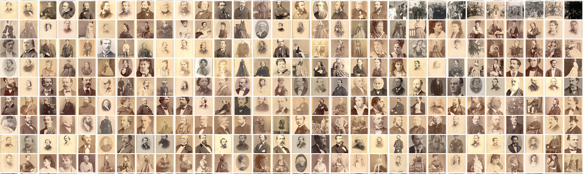
A common solution to this problem is to load an “image atlas”, or montage of small images combined into a single larger image:
One can then use the montage the way that performance-minded sites like Google use spritesheets. If you have ImageMagick installed, you can create one of these montages with the montage command:
# download directory of images
wget https://s3.amazonaws.com/duhaime/blog/tsne-webgl/data/100-imgs.tar.gz
tar-zxf 100-imgs.tar.gz
# create a file that lists all files to be include in the montagels 100-imgs/*> images_to_montage.txt
# create single montage image from images in a directory
montage `cat images_to_montage.txt`-geometry +0+0 -background none -tile 10x 100-img-atlas.jpg
The last command will create an image atlas with 10 images per column and no padding between the images in the atlas. The sample directory 100-imgs.tar.gz contains 100 images, and the -tile argument in the montage command indicates ouput atlas should have 10 columns, so the command above will generate a 10x10 grid of size 1280px by 1280px.
Let’s load the image atlas into a Three.js scene:
// Create a texture loader so we can load the image filevarloader=newTHREE.TextureLoader();// Load an image file into a custom materialvarmaterial=newTHREE.MeshBasicMaterial({map:loader.load('https://s3.amazonaws.com/duhaime/blog/tsne-webgl/data/100-img-atlas.jpg')});
Once the image atlas is loaded in, we’ll want to create some helper objects that identify the size of the atlas and its sub images. Those helper objects can then be used to calculate the vertex uvs of each face in a geometry:
// Identify the subimage size in pxvarimage={width:128,height:128};// Identify the total number of cols & rows in the image atlasvaratlas={width:1280,height:1280,cols:10,rows:10};
The custom geometry example above used four vertices and two faces to render a single image. To represent all 100 images from the image atlas, we can create four vertices and two faces for each of the 100 images to be displayed. Then we can associate the proper region of the image atlas material with each of the geometry’s 200 faces:
// Create a helper function that returns an int {-700,700}.// We'll use this function to set each subimage's x and// y coordinate positionsfunctiongetRandomInt(){varval=Math.random()*700;returnMath.random()>0.5?-val:val;}// Create the empty geometryvargeometry=newTHREE.Geometry();// For each of the 100 subimages in the montage, add four// vertices (one for each corner), in the following order:// lower left, lower right, upper right, upper leftfor(vari=0;i<100;i++){// Create x, y, z coords for this subimagevarcoords={x:getRandomInt(),y:getRandomInt(),z:-400};geometry.vertices.push(newTHREE.Vector3(coords.x,coords.y,coords.z),newTHREE.Vector3(coords.x+image.width,coords.y,coords.z),newTHREE.Vector3(coords.x+image.width,coords.y+image.height,coords.z),newTHREE.Vector3(coords.x,coords.y+image.height,coords.z));// Add the first face (the lower-right triangle)varfaceOne=newTHREE.Face3(geometry.vertices.length-4,geometry.vertices.length-3,geometry.vertices.length-2)// Add the second face (the upper-left triangle)varfaceTwo=newTHREE.Face3(geometry.vertices.length-4,geometry.vertices.length-2,geometry.vertices.length-1)// Add those faces to the geometrygeometry.faces.push(faceOne,faceTwo);// Identify this subimage's offset in the x dimension// An xOffset of 0 means the subimage starts flush with// the left-hand edge of the atlasvarxOffset=(i%10)*(image.width/atlas.width);// Identify the subimage's offset in the y dimension// A yOffset of 0 means the subimage starts flush with// the top edge of the atlasvaryOffset=Math.floor(i/10)*(image.height/atlas.height);// Use the xOffset and yOffset (and the knowledge that// each row and column contains only 10 images) to specify// the regions of the current imagegeometry.faceVertexUvs[0].push([newTHREE.Vector2(xOffset,yOffset),newTHREE.Vector2(xOffset+.1,yOffset),newTHREE.Vector2(xOffset+.1,yOffset+.1)]);// Map the region of the image described by the lower-left,// upper-right, and upper-left vertices to `faceTwo`geometry.faceVertexUvs[0].push([newTHREE.Vector2(xOffset,yOffset),newTHREE.Vector2(xOffset+.1,yOffset+.1),newTHREE.Vector2(xOffset,yOffset+.1)]);}// Combine the image geometry and material into a meshvarmesh=newTHREE.Mesh(geometry,material);// Set the position of the image mesh in the x,y,z dimensionsmesh.position.set(0,0,0)// Add the image to the scenescene.add(mesh);
Rendering that scene produces a crazy little scatterplot of images:
Here we represent one hundred images with just a single mesh! This is much better than giving each image its own mesh, as it reduces the number of required draw calls by two orders of magnitude. It’s worth noting, however, that eventually one does need to create additional meshes. A number of graphics devices can only handle 2^16 vertices in a single mesh, so if you need your scene to run on a wide range of devices it’s best to ensure each mesh contains 65,536 or fewer vertices.
Using Multiple Atlas Files
Having discovered how to visualize multiple images with a single mesh, we can now scale up the image collection size dramatically.
One way to crank up the number of visualized images is to squeeze more images into the image atlas. As it turns out, however, the largest texture size supported by many devices is 2048 x 2048px, so the code below will stick to atlas files of that size.
For the examples below, I took roughly 20,480 images, resized each to 32px thumbs, then used the montage technique discuss above to build the following atlas files: 1, 2, 3, 4, 5. Once those atlas files are loaded onto a static file server, one can load each atlas into a scene with a simple loop:
// Create a store that maps each atlas file's index position// to its materialvarmaterials={};// Create a texture loader so we can load the image filevarloader=newTHREE.TextureLoader();for(vari=0;i<5;i++){varurl='https://s3.amazonaws.com/duhaime/blog/tsne-webgl/data/atlas_files/32px/atlas-'+i+'.jpg';loader.load(url,handleTexture.bind(null,i));}// Callback function that adds the texture to the list of textures// and calls the geometry builder if all textures have loadedfunctionhandleTexture(idx,texture){materials[idx]=newTHREE.MeshBasicMaterial({map:texture})if(Object.keys(materials).length===5){document.querySelector('#loading').style.display='none';buildGeometry();}}
The buildGeometry function will then create the vertices and faces for the 20,000 images within the atlas files. Once those are set, one can pump those geometries into some meshes and add the meshes to the scene (click the Codepen link for the full code update):
So far we’ve used random coordinates to place images within a scene. Let’s now position images near other similar-looking images. To do so, we’ll create vectorized representations of each image, project those vectors down into a 2D embedding, then use each image’s position in the 2D coordinate space to position the image in the Three.js scene.
Generating TSNE Coordinates
First things first, let’s create a vector representation of each image. If you have tensorflow installed, you can create vectorized representations of each image in 100-imgs by running:
# download a script that generates vectorized representations of images
wget https://gist.githubusercontent.com/duhaime/2a71921c9f4655c96857dbb6b6ed9bd6/raw/0e72c48e698395265d029fabad0e6ab1f3961b26/classify_images.py

# install a dependency for process management
pip install psutil

# run the script on a glob of images
python classify_images.py '100-imgs/*'
This script will generate one image vector for each image in 100-imgs/. We can then run the following script to create a 2D TSNE projection of those image vectors:
# create_tsne_projection.py
fromsklearn.manifoldimportTSNEimportnumpyasnpimportglob,json,os# create datastores
image_vectors=[]chart_data=[]maximum_imgs=20480# build a list of image vectors
vector_files=glob.glob('image_vectors/*.npz')[:maximum_imgs]forc,iinenumerate(vector_files):image_vectors.append(np.loadtxt(i))print(' * loaded',c+1,'of',len(vector_files),'image vectors')# build the tsne model on the image vectors
model=TSNE(n_components=2,random_state=0)np.set_printoptions(suppress=True)fit_model=model.fit_transform(np.array(image_vectors))# store the coordinates of each image in the chart data
forc,iinenumerate(fit_model):chart_data.append({'x':float(i[0]),'y':float(i[1]),'idx':c})withopen('image_tsne_projections.json','w')asout:json.dump(chart_data,out)
Running that TSNE script on your image vectors will generate a JSON file in which each input image is mapped to x and y coordinate values:
Given the JSON file with those TSNE coordinates, all we need to do is iterate over each item in the JSON file and position the image in that index position accordingly.
To load a JSON file using the Three.js library, we can use a FileLoader:
// Create a store for image position informationvarimagePositions=null;varloader=newTHREE.FileLoader();loader.load('https://s3.amazonaws.com/duhaime/blog/tsne-webgl/data/image_tsne_projections.json',function(data){imagePositions=JSON.parse(data);// Build the geometries if all atlas files are loadedconditionallyBuildGeometries()})
We can then use the index position of each item in that JSON file to identify the appropriate atlas file and x, y offsets for a given image. To do so, we’ll need to store each material by its index position:
// Create a texture loader so we can load the image filevarloader=newTHREE.TextureLoader();for(vari=0;i<5;i++){varurl='https://s3.amazonaws.com/duhaime/blog/tsne-webgl/data/';url+='atlas_files/32px/atlas-'+i+'.jpg';// Pass the texture index position to the callback functionloader.load(url,handleTexture.bind(null,i));}// Callback function that adds the texture to the list of textures// and calls the geometry builder if all textures have loadedfunctionhandleTexture(idx,texture){materials[idx]=newTHREE.MeshBasicMaterial({map:texture})conditionallyBuildGeometries()}// If the textures and the mapping from image idx to positional information// are all loaded, create the geometriesfunctionconditionallyBuildGeometries(){if(Object.keys(materials).length===5&&imagePositions){document.querySelector('#loading').style.display='none';buildGeometry();}}
Then buildGeometry() can then pass the index position of each atlas i and the index position of each image within a given atlas j to getCoords(), a function that returns the given image’s x and y coordinates:
// Identify the total number of cols & rows in the image atlasvaratlas={width:2048,height:2048,cols:64,rows:64};// Create a new mesh for each texturefunctionbuildGeometry(){for(vari=0;i<5;i++){// Create one new geometry per atlasvargeometry=newTHREE.Geometry();for(varj=0;j<atlas.cols*atlas.rows;j++){varcoords=getCoords(i,j);geometry=updateVertices(geometry,coords)geometry=updateFaces(geometry)geometry=updateFaceVertexUvs(geometry,j)}buildMesh(geometry,materials[i])}}// Get the x, y, z coords for the subimage in index position j// of atlas in index position ifunctiongetCoords(i,j){varidx=(i*atlas.rows*atlas.cols)+j;varcoords=imagePositions[idx];coords.x*=1200;coords.y*=600;coords.z=(-200+j/100);returncoords;}
Adding Controls
In addition to setting the image positions, we can add some controls to the scene that allow users to zoom in or out. An easy way to do so is to add the pre-packaged trackball controls as an additional JavaScript dependency. Then we can call the control’s constructor and update the controls both on window resize events and inside the main render loop to keep the controls up to date with the application state:
/**
* Add Controls
**/varcontrols=newTHREE.TrackballControls(camera,renderer.domElement);/**
* Handle window resizes
**/window.addEventListener('resize',function(){camera.aspect=window.innerWidth/window.innerHeight;camera.updateProjectionMatrix();renderer.setSize(window.innerWidth,window.innerHeight);controls.handleResize();});/**
* Render!
**/// The main animation functionfunctionanimate(){requestAnimationFrame(animate);renderer.render(scene,camera);controls.update();}animate();
The result is an interactive visualization of the images in a 2D TSNE projection:
We’ve now achieved a basic TSNE map with Three.js, but there’s much more that could be done to improve a user’s experience of the visualization. In particular, within the extant plot:
* Users get no indication of load progress
* Users can't see details within the small images
* Users have no guide through the visualization
To see how our team resolved those challenges, feel free to visit the live site or the GitHub repository with the full source code. Otherwise, if you’re working on something similar, feel free to send me a note or a comment below–I’d love to see what you’re building.
* * *
I want to thank Cyril Diagne, a lead developer on the spectacular Google Arts Experiments TSNE viewer, for generously sharings ideas and optimization techniques that we used to build our own TSNE viewer.


