Adventures in Drone Photogrammetry Using Rust and Machine Learning
Posted 11/14/2021
[tl;dr] I took a picture of a tarp with a drone. Using basic photogrammetry, I estimated the area of the picture, used machine learning to segment the tarp in the image, and got an tarp area of 3.86 m2 compared to the actual area of 3.96 m2 (~4% error). I wrote the whole thing in Rust; the code is on Github here and data is here.
Not too long ago, I decided to leave my job as a research engineer at UC Santa Barbara, and take some time off to rest, recharge, and explore on a few things that I've been interested in but haven't had the time to try out until now. Unfortunately, the downside of leaving a position where I got to work with robots on a regular basis is that, well, I no longer had any robots to work with. To help with some of the painful robot withdrawal, I purchased a drone, and started seeing what possibilities it might offer. One of those was photogrammetry, or the measurement of objects through the interpretation of images. To be clear, I'm not an expert in the field, but it was a fun experiment and I think the results potentially offer some neat applications in the future.
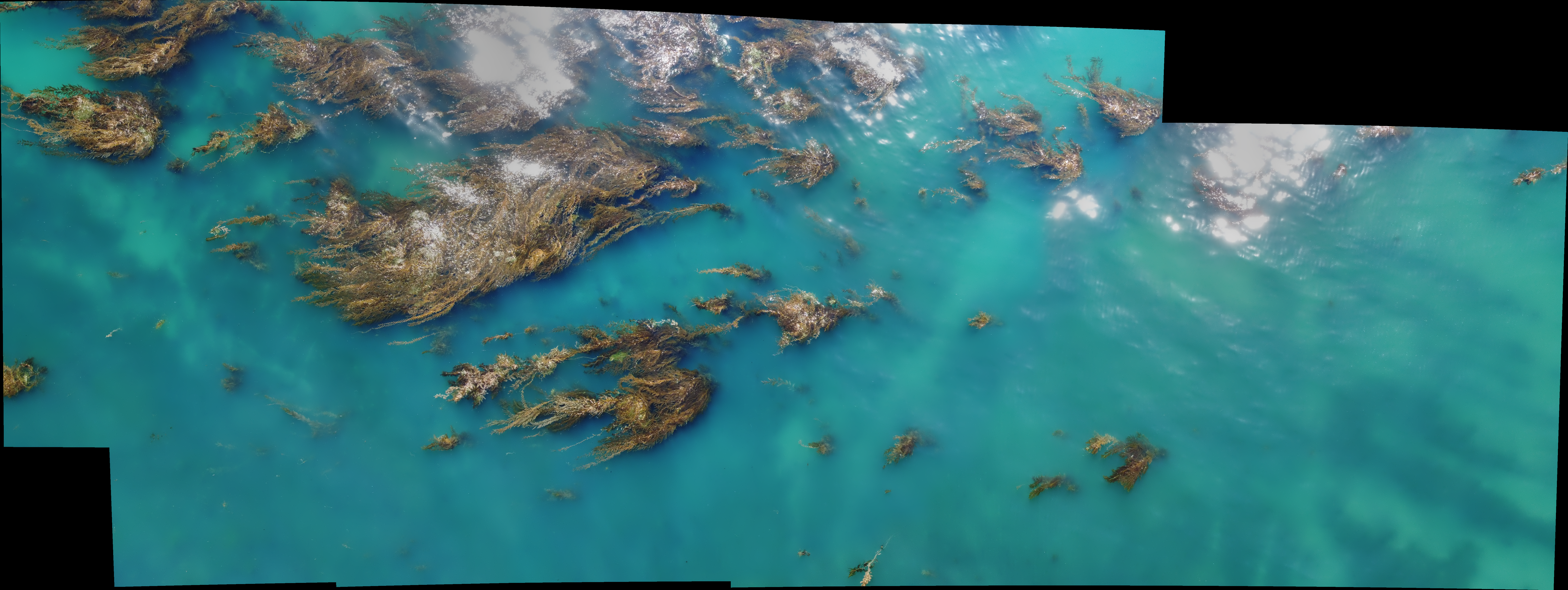
Why would we want to measure things from a drone photo? Well, besides the somewhat honest answer of "just because", it turns out that there's some neat applications in areas like environmental monitoring. For example, wetlands play a really important role in carbon sequestration, but usually are also dynamic environments. I've helped support scientists doing work like this on kelp forests, but there's also potential applications in other ecosystems like castorid wetlands (beaver dams).
Before we can measure something cool like the area of a beaver pond, however, we need to set up a control to make sure that we can accurately measure things from the air.
"Wait, aren't there off-the-shelf products built for this sort of thing?"
Why yes, you clear-eyed devil, there in fact are. Unfortunately, they're pretty expensive and I just left my job. Besides, I've got some spare time on my hands, and I thought it might be more interesting to build it myself, and maybe learn something along the way. That said, while I have spent some time playing around with building my own drone from scratch, for this project I'm using a DJI Mini 2. I think this is a nice middle-ground; the Mini 2 is easy to fly, under 250 grams (so doesn't require FAA registration), but still has ~30 minute flight time and a camera capable of high-res 4K stills. However, the Mini 2 is API-limited, at least for the moment. Unlike the DJI pro-focused offerings, there's not a developer API available for the Mini 2, and as a consumer model, the professional mapping software offered for platforms like the DJI Phantom with features like auto-mapping and waypoint missions aren't compatible. At the moment, this isn't a huge issue (we'll be checking our photogrammetry method using a single image), but on larger areas in the future, we'll start relying on OpenCV to stitch together individual images into larger landscape-level panoramas.
If you don't care about drones and want to move right into the photogrammetry part, feel free to click here.
Flight
A drone flight using the Mini 2 is fairly basic once the initial pairing between the contoller and the drone has taken place. In order to fly, we need the drone, the controller, a charged battery, a μSD card, and a smartphone running the DJI Pilot app. After connecting the phone to the controller over a USB-C port and turning on the both the drone and the controller, a live video feed should start up pretty soon afterwards.

DJI Mini 2 flight hardware
Flight after pairing is fairly simple; simply set the drone down in a flat location a few meters away with the camera facing away from you (and anyone else in the vicinity, safety first), and double-tap the "Begin Flight" button on the app. The Mini 2 will automatically start its propellers and lift itself into a hover at around 1.2 m off the ground. Importantly, the zero position (where the drone considers 0.0 m) is based on the initial flight elevation, not it's actual height over ground. This is important in areas where we might start flying on a cliff or other elevated location which, for example, we might want to do while surveying a coastal ocean location.
The goal of this flight is to take a top-down photograph at a known height of an easily-identified target with a known area. By doing this, we'll be able to test our photogrammetry method for estimating areas will result in an an accurate value. Ideally, we'll also do this from various heights to make sure that we're not missing some sort of non-linearity that will accidentally show up in the future when flying over targets at a different altitude than during this test.
In order to accomplish this, I started by laying out a silver tarp on a soccer field, where the difference in color should make it fairly easy to discriminate. Second, the drone itself was flown up to an altitude of 9.9 m, and the camera turned at a 90° angle, nominally pointing directly down. The Mini 2 doesn't have an easy way to revisit flight logs afterwards, so checking height before taking the picture is important. Similarly, the specified height above 10 m only changes in 1 meter intervals, vs. 0.1 meter intervals before 10 m. We're interested in having as accurate a height estimate as possible, so while it's possible to guess the approximate height based on checking for the transition point between, say, 19 m and 20 m (which would put the height at around 19.9 meters), the we'll take what we can get at the start.

Tarp image taken at 9.9 m altitude
A Brief Introduction to Photogrammetry
At a high level, photogrammetry is based on angles, distances, and right triangles. Below is a(n admittedly rough) sketch of how this works.

Basic photogrammetric geometry sketch
The drone sits at an altitude , where it takes a picture at a certain resolution. We intuitively know that this picture has a finite area--that is, the rectangle of pixels that makes up the pictures only covers a certain amount of area. Even better, since we know the resolution of our picture ("4K" means we get a 4000 x 2250 pixel image), we can approximate the area covered by each pixel individually, and the sum the total of the "tarp" pixels to get the an estimate of the actual area.
But how much area does our image cover? That depends mainly on two things: the height of the drone, and the lens angle of the camera. The lens angle is a built-in property of the drone; we can pull it from the manufacturer specs, where for the Mini2, . From there, we'll use some of that high school trigonometry we were never sure we'd use to solve for the length of the far side of the triangle. Note that in order to form the right triangle, we're actually using , which only gives us half of the picture's actual width, .
    fn area_from_pixels(drone_height: f64,
                        tarp_pixels: usize,
                        scaling_factor: f64) -> f64 {
        // DJI Mini 2 camera specs: https://www.dji.com/mini-2/specs
        // FOV: 83°
        // Focus range: 1 m to ∞
        // Image resolution: 4000x2250

        // We'll come back to this number later
        let definitely_not_a_fudge_factor = 0.5;
        let lens_angle_v: f64 =
            (definitely_not_a_fudge_factor * 83f64).to_radians() / 2.0;
        let lens_angle_h: f64 = 83f64.to_radians() / 2.0;

        // Vertical edge length of the image frame is real distance at `d` meters
        let l_v = 2.0 * drone_height * lens_angle_v.atan();
        let l_h = 2.0 * drone_height * lens_angle_h.atan();

        let frame_area = l_v * l_h;

        let w = 4000.0 * scaling_factor; // # of pixels on the x-axis
        let h = 2250.0 * scaling_factor; // # of pixels on the y-axis
        let pixel_area = frame_area / (w * h); // Area per pixel in meters
        // Fun fact: Rust formatting includes support for scientific notation!
        println!("Pixel area: {:.2e} m^2", pixel_area);

        let est_tarp_area = tarp_pixels as f64 * pixel_area;
        est_tarp_area
    }
How (Not To) Segment An Image
At this point, we've got an estimate for the area covered by each pixel; the next step is to try to calculate the number of pixels that are assigned to the the tarp in the image. Once we have that, we can simply multiply the two together:
and we'll have our answer. But how to count the pixels in the tarp?
There are a few ways that we could do this; to start, it's pretty easy to open up GIMP and pull out the Measure utility. Since the tarp is rectangular, all it would take is a measurement along each axis. Of course, this approach is pretty unlikely to work on anything besides rectangles; it doesn't generalize very well.

Measuring the tarp in GIMP
We could also use something like a color filter. Each pixel in the image is represented as an image::Rgba([r, g, b, α]) data structure. By iterating over each one, we could check to see if it matches a set of rules that we provide that would prefer the tarp's pixels over all others.
For example, we know that the tarp is silver, while the rest of the field is green. As a result, the ratio of Green to Blue should be much higher on the grass than the tarp. So we, could create a function like
  /// Check if a pixel is grey based on green/blue ratio
  #[inline]
  fn is_grey(pixel: Rgba<u8>, threshold: f64) -> bool {
      if (pixel[1] as f64 / pixel[2] as f64) > threshhold {
          true
      }
      else {
          false
      }
  }
The problem with simple color filters is that they tend not to end up being so simple. A single rule rarely takes care of everything, so you start adding conditionals, which are then based on things like lighting or location, so you add more conditionals, but then some rules conflict with others so you add more conditionals to resolve those, and so on forever until you give up and go live in a monastery for a while to contemplate the infinite possibilities created by the universe's fickle nature. Ahem.
Anyway, while this might work for a one-off, it's an approach that rarely ends up being more flexible than just coloring in the image yourself and going from there.
Speaking on coloring in, if we knew we were going to be doing a ton of this kind of characterization in the future, we might want to try something like semantic segmentation using a convolutional neural network. In fact, you can get decent results with relatively little training data using this approach, especially if you use one of the pre-built solutions like FastAI's Segmentation API.
However, unless you already have a pipeline set up for it, annotating data by hand may not be worth it for only a few pictures, at which point you'll either need to rent a GPU from a cloud provider or spend the money on one yourself in order to have enough room to fit an effective training network in anyway.
Image Segmentation with linfa and DBSCAN
In this case, the core task that we're working on is separating out a localized group of pixels that display a significant color difference over the other pixels in the image.
This just happens the is the sort of sweet spot where a clustering algorithm might come in handy. One of the most of common of these is DBSCAN, or the "Density-Based Spatial Clustering with Noise." While I'm not going to explain how it works here, it functionally does a really good job at automatically identifying groups of related data, while also filtering out data that is unrelated to any of those groups. In addition, DBSCAN often does a nice job while dealing with not-so-structured data, which is an asset when dealing with real-world image data. If you are interested in a more in-depth exploration, feel free to take a look at the chapter I wrote about it for the Rust-ML Book here.
The first thing we'll do is open the image file with the image library, then resize the image. Resizing isn't necessary, but is often practical in order to reduce iteration time. I'd recommend trying a scaling factor to start.
    let img = image::open(path)?;
    let (w, h) = img.dimensions(); // (u32, u32)
    // Resize the image based on a [0.0, 1.0] scaling factor
    // Smaller images (smaller scales) will be faster, but with
    // less resolution
    let img = resize(
        &img,
        (w as f64 * scaling_factor) as u32,
        (h as f64 * scaling_factor) as u32,
        FilterType::Triangle, // Different filters have different effects
    );
Once the image is resized, we'll want to convert it into a form that can be easily processed by linfa, a Rust machine learning library akin to scikit-learn. In this case, we'll flatten it out, where each pixel is a new row in the form [x, y, r, g, b], to create an ndarray::Array2<f64> array.
From there, we can call the linfa-clustering::AppxDbscan algorithm (similar to the vanilla DBSCAN algorithm, but which often runs a little more quickly), and supply it with a couple of hyperparameters. You may need to play with the tolerance parameter a little bit before getting it right.
    // Convert this image into an Array2<f64> array with [x,y,r,g,b] rows
    for y in 0..h {
        for x in 0..w {
            let pixel = img.get_pixel(x, y);
            let num = (y * w) + x;

            array[[num as usize, 0]] = x as f64;
            array[[num as usize, 1]] = y as f64;
            array[[num as usize, 2]] = pixel[0] as f64;
            array[[num as usize, 3]] = pixel[1] as f64;
            array[[num as usize, 4]] = pixel[2] as f64;
        }
    }

    let min_points = 500;
    // Since the tarp is local, we'll use all [x,y] coordinates as well,
    // but we could only evaluate based on color using array.slice(s![.., 2..])
    let clusters = AppxDbscan::params(min_points)
        .tolerance(tolerance) // Tolerance param is supplied in fn args
        .transform(&array.slice(s![.., ..]))?;
Depending on the hyperparameters, clustering may take anywhere from a few seconds to a few minutes, and should scale geometrically with the size of the image. The returned value is a vector of assigned clusters, with a total length equal to the number of rows in the original array. We'll iterate of this list, and depending on the cluster value, write one of several pixel options to the [x, y] position of that pixel. Critically, each time that we get a tarp pixel (assigned the second-largest cluster), we'll add to a running count and color it RED.
    let mut count = 0;
    for i in 0..array.shape()[0] {
        let x = array[[i, 0]] as u32;
        let y = array[[i, 1]] as u32;
        let pixel = img.get_pixel(x, y);
        match clusters[i] {
            Some(0) => {
                // If it's part of the background, keep the original pixel
                new_img.put_pixel(x, y, *pixel);
            }
            Some(1) => {
                // Color tarp-assigned pixels RED
                new_img.put_pixel(x, y, Rgba([255, 0, 0, 255]));
                count += 1;
            }
            // In DBSCAN, not all pixels are assigned a cluster
            // Color unassigned pixels BLUE
            None => {
                new_img.put_pixel(x, y, Rgba([0, 0, 255, 255]));
            }
            _ => {
                // Depending on our selected hyperparameters, we could
                // potentially get a scattering of smaller clusters
                // Color small clusters YELLOW, should they occur
                new_img.put_pixel(x, y, Rgba([255, 170, 29, 255]));
            }
        }
    }
Results
Summary:
At 9.9 m height, this method estimated an area of 3.86 m2, vs. 3.96 m2 actual. This represents an error of approximately 3.0%.
At 20 m height, this method estimated an area of 3.92 m2, vs. 3.96 m2 actual. This represents an error of approximately 1.5%.
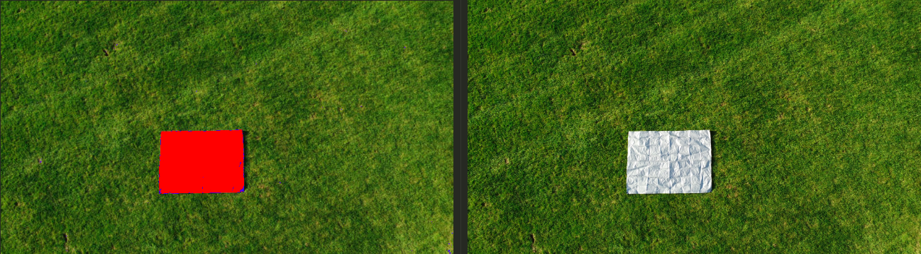
After clustering, we can see that the algorithm has done its job well; the tarp is almost completely covered with red pixels, and there are very few falsely-identified pixels elsewhere. One interesting result is the assignment of a None label to the perimeter of the tarp. I think that this is due to the shadow created along the edge, where the tarp is not sitting fully flat along the ground.

Original tarp photo vs. clustered result (h = 9.9 m)
For the above result, the segmentation process was run with hyperparams of (scaling_factor, tolerance) = (0.20, 20.0), resulting in 16253 tarp pixels and an estimated tarp area of 3.86 m2. Compared to the actual area of 3.96 m2, this represents an error of approximately 3.0%

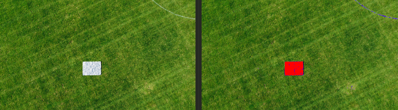
Original tarp photo vs. clustered result (h = 20 m)
Using the same hyperparameters with a height of 20 m, 4049 tarp pixels were estimated and a resulting tarp area of 3.86 m2, or 1.5% error compared to the 3.96 m2 actual area. It's also worth noting that a white painted line was present in the upper right corner of the 20 m image, and demonstrates the value of using DBSCAN instead of something like naive color filtering; many pixels in that line were noted as not belonging to the standard background, but none were assigned to the tarp itself.
As a result, I believe that this method demonstrates solid proof-of-concept for performing basic photogrammetry from a low-cost consumer-grade drone like the DJI Mini 2. It also demonstrates the ability of using Rust data science tools to perform data analysis with relatively low overhead.
Next Steps, or "Hey, wait, what was 'fudge factor' from that code snippet above?"
Ah, I can't get one by you, ya opalescent tree shark. Yes, in the area estimation code above, there's a variable called definitely_not_a_fudge_factor, where I multiply the angle of the horizontal lens angle by an additional 0.5. Based on the numbers we have, this is not in line with a purely first-principles approach. However, I think there's a fair justification for doing this.
    // ↓ (this thing)
    let definitely_not_a_fudge_factor = 0.5;
    let lens_angle_v: f64 =
        (definitely_not_a_fudge_factor * 83f64).to_radians() / 2.0;
First, I should say that I'm mostly doing this because It Seems To Work™. Second, cameras that are involved in photogrammetry tend to have more than a single number reported for their field-of-view angles, where the horizontal and vertical angles have different values. Take a look at the specs of a StereoLabs ZED camera, for instance. This isn't the case in the Mini 2's documentation; it only has a single value of 83°. Especially considering that the resulting images don't have a 1:1 aspect ratio at any resolution (it's actually a 16:9 ratio), I suspect there's some missing information here. In general, it would be ideal to determine the actual effective field of views, as well as correct for image distortion common to cameras like this one.
We could instead do a simple ratio for this correction factor; a ratio of 9/16 is technically 0.5625. However, when I was testing this, no matter how I measured the size of the tarp (in GIMP, using various DBSCAN hyperparams, etc.), I was consistently getting too high an area (closer to 8-10% error over actual rather than 2-4%). Since I'm missing this information anyway, I unscientifically dropped that ratio to 2:1 instead. Considering the lack of precision in altitude data (maybe the measurement is slightly biased?) I don't consider this particularly egregious, but it is something worth calling out and keeping an eye on in the future data. Having a control area in place would be a prudent check on this in future datasets.
In addition, this could be worked into more formal estimates for the variation; right now we're reporting the error percentages based on a single value. Using additional tests, as well as considering individual contribution sources of error like altitude, it would be possible to produce a more formal uncertainty analysis for this measurement.
Additional Future Work
Besides keeping an eye on the effect of that adjustment factor for θv, a good next step would be evaluating the effects of panorama stitching on this process. Especially for applications like environmental monitoring, a single photo rarely covers enough ground to be truly useful, and as a drone get higher up, the resolution of the images necessarily decrease. As a result, stitching together a number of low-altitude images could allow us to run this kind of segmentation-for-area process on larger, more complex targets.
I've actually already put together a prototype for this using OpenCV's Python bindings. There is an OpenCV bindings for Rust (opencv-rust), but it would be really cool to use a native Rust library to do this. While developers in the Rust-CV organization has mentioned that this will eventually on their roadmap, several required elements like homography estimators need to be implemented first. Similarly, using OpenCV's functions for calibrating the camera and measuring/correcting for the aforementioned distortion would be possible, although likely difficult without dropping back down in the native library. In the meantime, scripting together those functions would be possible (or I could port the whole thing over to Python). For specific problems, using a semantic segmentation model to identify target pixels would also be an interesting challenge.
This was a lot of fun to explore, and I have to admit I'm looking forward to getting out into more interesting places for flights in the future. If you have any questions, comments, constructive feedback, corrections, or interpretive dances, please feel free to reach out to me over email. Thanks for stopping by!
Thanks to Geordan Worley (vadix) for taking the time to review a draft of this and give me some excellent feedback! Any mistakes are, of course, only mine.